Create minimum spanning network of selected populations using Bruvo's distance.
Source:R/bruvo.r
bruvo.msn.RdCreate minimum spanning network of selected populations using Bruvo's distance.
bruvo.msn(
  gid,
  replen = 1,
  add = TRUE,
  loss = TRUE,
  mlg.compute = "original",
  palette = topo.colors,
  sublist = "All",
  exclude = NULL,
  blacklist = NULL,
  vertex.label = "MLG",
  gscale = TRUE,
  glim = c(0, 0.8),
  gadj = 3,
  gweight = 1,
  wscale = TRUE,
  showplot = TRUE,
  include.ties = FALSE,
  threshold = NULL,
  clustering.algorithm = NULL,
  ...
)
Arguments
| gid | a |
|---|---|
| replen | a |
| add | if |
| loss | if |
| mlg.compute | if the multilocus genotypes are set to "custom" (see
|
| palette | a |
| sublist | a |
| exclude | a |
| blacklist | DEPRECATED, use exclude. |
| vertex.label | a |
| gscale | "grey scale". If this is |
| glim | "grey limit". Two numbers between zero and one. They determine
the upper and lower limits for the |
| gadj | "grey adjust". a positive |
| gweight | "grey weight". an |
| wscale | "width scale". If this is |
| showplot | logical. If |
| include.ties | logical. If |
| threshold | numeric. By default, this is |
| clustering.algorithm | string. By default, this is |
| ... | any other arguments that could go into plot.igraph |
Value
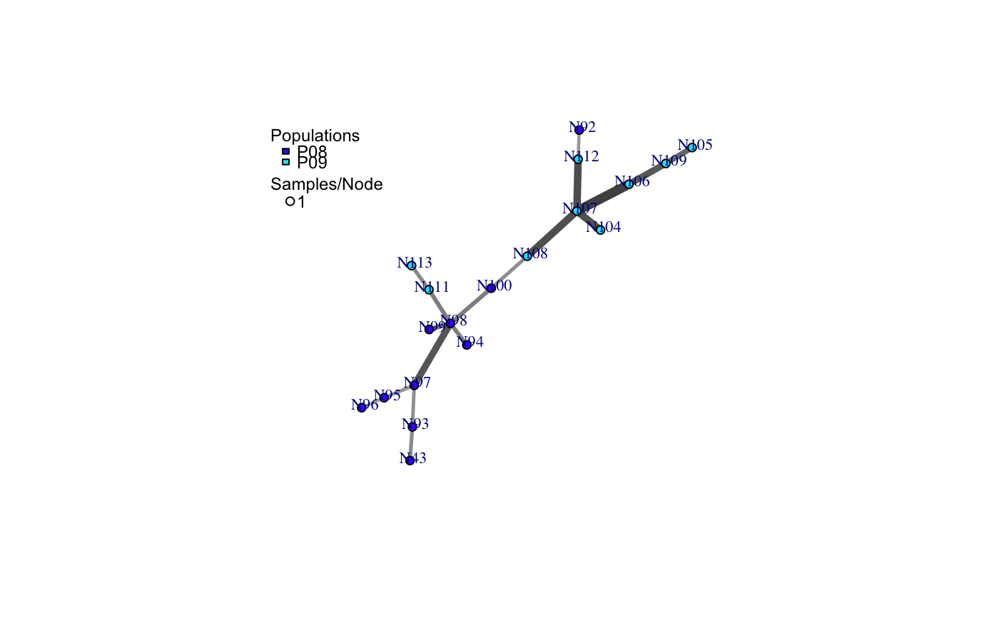
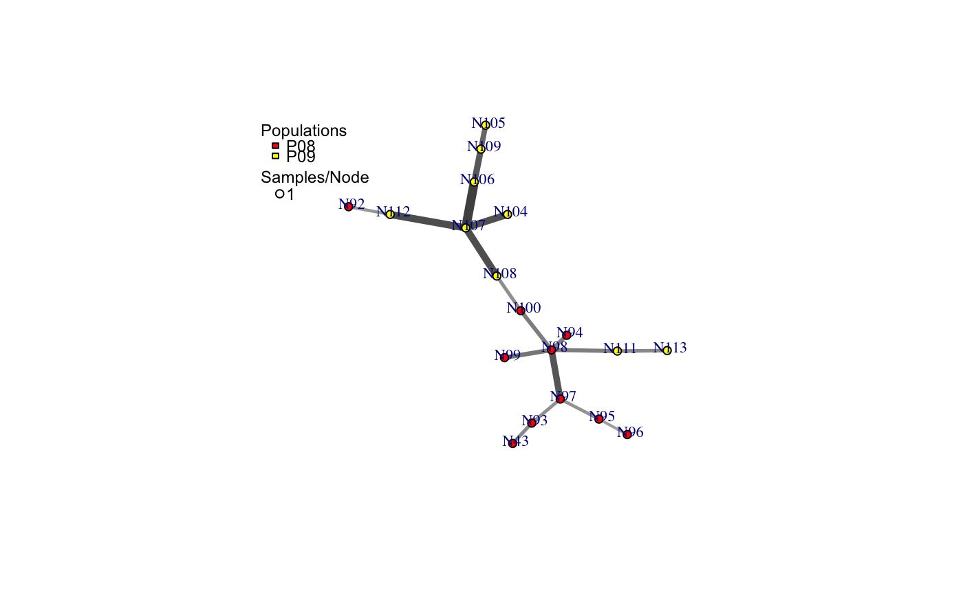
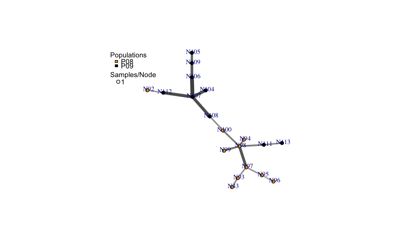
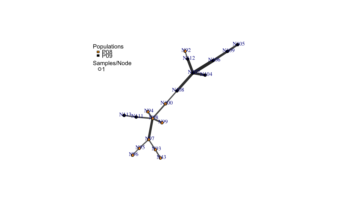
a minimum spanning network with nodes corresponding to MLGs within the data set. Colors of the nodes represent population membership. Width and color of the edges represent distance.
a vector of the population names corresponding to the vertex colors
a vector of the hexadecimal representations of the colors used in the vertex colors
Details
The minimum spanning network generated by this function is generated
via igraph's minimum.spanning.tree. The resultant
graph produced can be plotted using igraph functions, or the entire object
can be plotted using the function plot_poppr_msn, which will
give the user a scale bar and the option to layout your data.
node sizes
The area of the nodes are representative of the number of samples. Because igraph scales nodes by radius, the node sizes in the graph are represented as the square root of the number of samples.
mlg.compute
Each node on the graph represents a different multilocus genotype.
The edges on the graph represent genetic distances that connect the
multilocus genotypes. In genclone objects, it is possible to set the
multilocus genotypes to a custom definition. This creates a problem for
clone correction, however, as it is very possible to define custom lineages
that are not monophyletic. When clone correction is performed on these
definitions, information is lost from the graph. To circumvent this, The
clone correction will be done via the computed multilocus genotypes, either
"original" or "contracted". This is specified in the mlg.compute
argument, above.
contracted multilocus genotypes
If your incoming data set is of the class genclone,
and it contains contracted multilocus genotypes, this function will retain
that information for creating the minimum spanning network. You can use the
arguments threshold and clustering.algorithm to change the
threshold or clustering algorithm used in the network. For example, if you
have a data set that has a threshold of 0.1 and you wish to have a minimum
spanning network without a threshold, you can simply add
threshold = 0.0, and no clustering will happen.
The threshold and clustering.algorithm arguments can also be
used to filter un-contracted data sets.
Note
Please see the documentation for
bruvo.distfor details on the algorithm.The edges of these graphs may cross each other if the graph becomes too large.
The nodes in the graph represent multilocus genotypes. The colors of the nodes are representative of population membership. It is not uncommon to see different populations containing the same multilocus genotype.
References
Ruzica Bruvo, Nicolaas K. Michiels, Thomas G. D'Souza, and Hinrich Schulenburg. A simple method for the calculation of microsatellite genotype distances irrespective of ploidy level. Molecular Ecology, 13(7):2101-2106, 2004.
See also
bruvo.dist, nancycats,
plot_poppr_msn, minimum.spanning.tree
bruvo.boot, greycurve poppr.msn
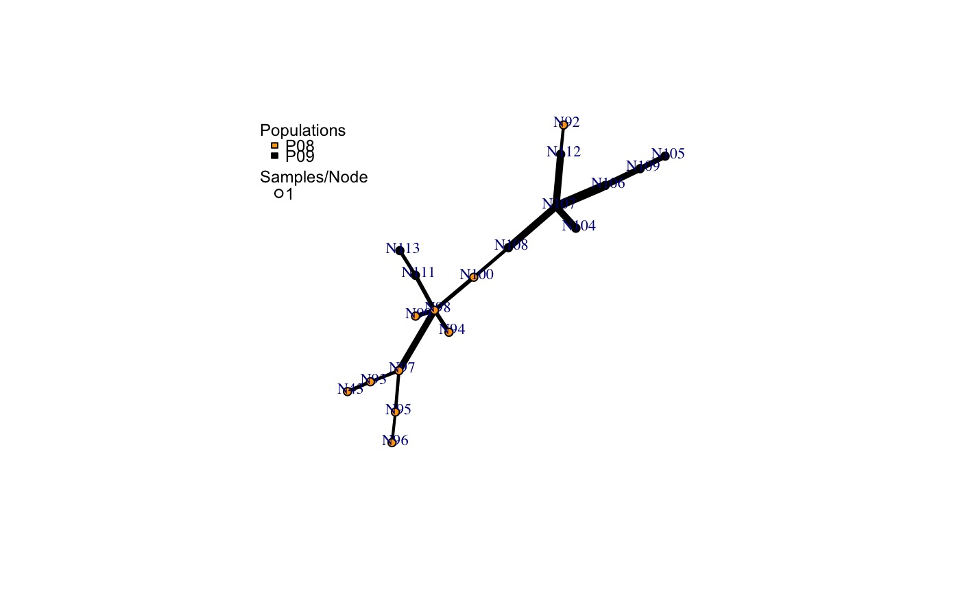
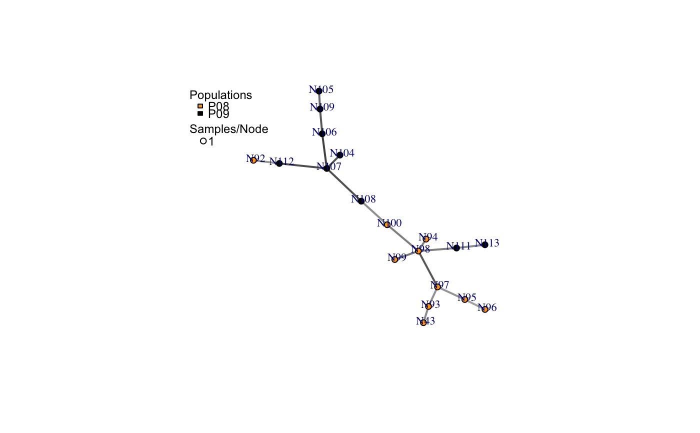
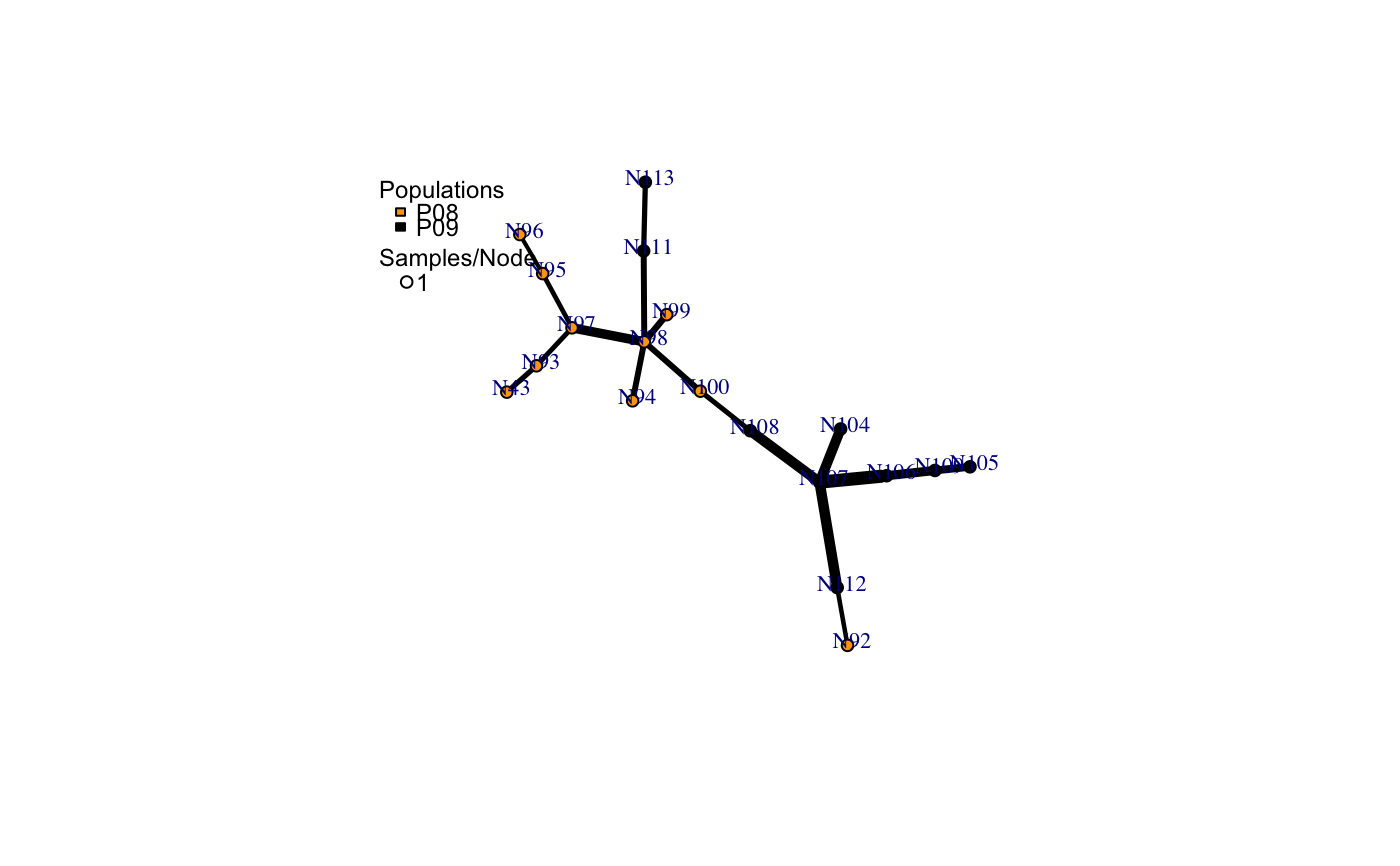
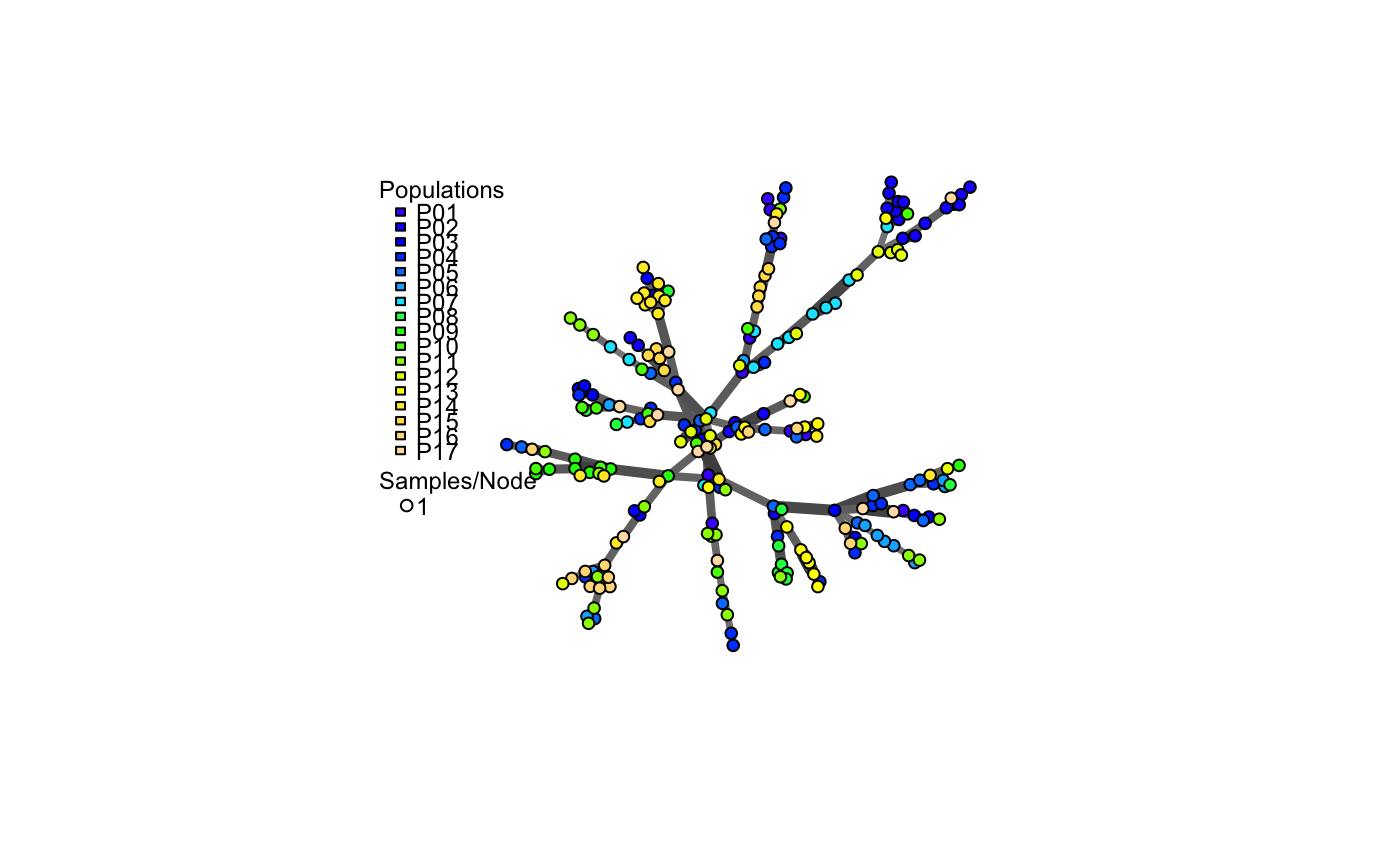
Examples
# Load the data set. data(nancycats) # View populations 8 and 9 with default colors. bruvo.msn(nancycats, replen = rep(2, 9), sublist=8:9, vertex.label="inds", vertex.label.cex=0.7, vertex.label.dist=0.4)#> $graph #> IGRAPH 71923d7 UNW- 19 18 -- #> + attr: name (v/c), size (v/n), shape (v/c), pie (v/x), pie.color #> | (v/x), color (v/c), label (v/c), weight (e/n), color (e/c), width #> | (e/n) #> + edges from 71923d7 (vertex names): #> [1] N43 --N93 N92 --N112 N94 --N98 N95 --N96 N95 --N97 N98 --N99 #> [7] N98 --N100 N98 --N97 N98 --N111 N100--N108 N93 --N97 N104--N107 #> [13] N105--N109 N106--N107 N106--N109 N107--N108 N107--N112 N111--N113 #> #> $populations #> [1] "P08" "P09" #> #> $colors #> P08 P09 #> "#4C00FF" "#00E5FF" #># \dontrun{ # View heat colors. bruvo.msn(nancycats, replen=rep(2, 9), sublist=8:9, vertex.label="inds", palette=heat.colors, vertex.label.cex=0.7, vertex.label.dist=0.4)#> $graph #> IGRAPH 7606b43 UNW- 19 18 -- #> + attr: name (v/c), size (v/n), shape (v/c), pie (v/x), pie.color #> | (v/x), color (v/c), label (v/c), weight (e/n), color (e/c), width #> | (e/n) #> + edges from 7606b43 (vertex names): #> [1] N43 --N93 N92 --N112 N94 --N98 N95 --N96 N95 --N97 N98 --N99 #> [7] N98 --N100 N98 --N97 N98 --N111 N100--N108 N93 --N97 N104--N107 #> [13] N105--N109 N106--N107 N106--N109 N107--N108 N107--N112 N111--N113 #> #> $populations #> [1] "P08" "P09" #> #> $colors #> P08 P09 #> "#FF0000" "#FFFF00" #># View custom colors. Here, we use black and orange. bruvo.msn(nancycats, replen=rep(2, 9), sublist=8:9, vertex.label="inds", palette = colorRampPalette(c("orange", "black")), vertex.label.cex=0.7, vertex.label.dist=0.4)#> $graph #> IGRAPH 94a14b0 UNW- 19 18 -- #> + attr: name (v/c), size (v/n), shape (v/c), pie (v/x), pie.color #> | (v/x), color (v/c), label (v/c), weight (e/n), color (e/c), width #> | (e/n) #> + edges from 94a14b0 (vertex names): #> [1] N43 --N93 N92 --N112 N94 --N98 N95 --N96 N95 --N97 N98 --N99 #> [7] N98 --N100 N98 --N97 N98 --N111 N100--N108 N93 --N97 N104--N107 #> [13] N105--N109 N106--N107 N106--N109 N107--N108 N107--N112 N111--N113 #> #> $populations #> [1] "P08" "P09" #> #> $colors #> P08 P09 #> "#FFA500" "#000000" #># View with darker shades of grey (setting the upper limit to 1/2 black 1/2 white). bruvo.msn(nancycats, replen=rep(2, 9), sublist=8:9, vertex.label="inds", palette = colorRampPalette(c("orange", "black")), vertex.label.cex=0.7, vertex.label.dist=0.4, glim=c(0, 0.5))#> $graph #> IGRAPH 9da823c UNW- 19 18 -- #> + attr: name (v/c), size (v/n), shape (v/c), pie (v/x), pie.color #> | (v/x), color (v/c), label (v/c), weight (e/n), color (e/c), width #> | (e/n) #> + edges from 9da823c (vertex names): #> [1] N43 --N93 N92 --N112 N94 --N98 N95 --N96 N95 --N97 N98 --N99 #> [7] N98 --N100 N98 --N97 N98 --N111 N100--N108 N93 --N97 N104--N107 #> [13] N105--N109 N106--N107 N106--N109 N107--N108 N107--N112 N111--N113 #> #> $populations #> [1] "P08" "P09" #> #> $colors #> P08 P09 #> "#FFA500" "#000000" #># View with no grey scaling. bruvo.msn(nancycats, replen=rep(2, 9), sublist=8:9, vertex.label="inds", palette = colorRampPalette(c("orange", "black")), vertex.label.cex=0.7, vertex.label.dist=0.4, gscale=FALSE)#> $graph #> IGRAPH 077fe52 UNW- 19 18 -- #> + attr: name (v/c), size (v/n), shape (v/c), pie (v/x), pie.color #> | (v/x), color (v/c), label (v/c), weight (e/n), color (e/c), width #> | (e/n) #> + edges from 077fe52 (vertex names): #> [1] N43 --N93 N92 --N112 N94 --N98 N95 --N96 N95 --N97 N98 --N99 #> [7] N98 --N100 N98 --N97 N98 --N111 N100--N108 N93 --N97 N104--N107 #> [13] N105--N109 N106--N107 N106--N109 N107--N108 N107--N112 N111--N113 #> #> $populations #> [1] "P08" "P09" #> #> $colors #> P08 P09 #> "#FFA500" "#000000" #># View with no line widths. bruvo.msn(nancycats, replen=rep(2, 9), sublist=8:9, vertex.label="inds", palette = colorRampPalette(c("orange", "black")), vertex.label.cex=0.7, vertex.label.dist=0.4, wscale=FALSE)#> $graph #> IGRAPH f5a8b2a UNW- 19 18 -- #> + attr: name (v/c), size (v/n), shape (v/c), pie (v/x), pie.color #> | (v/x), color (v/c), label (v/c), weight (e/n), color (e/c), width #> | (e/n) #> + edges from f5a8b2a (vertex names): #> [1] N43 --N93 N92 --N112 N94 --N98 N95 --N96 N95 --N97 N98 --N99 #> [7] N98 --N100 N98 --N97 N98 --N111 N100--N108 N93 --N97 N104--N107 #> [13] N105--N109 N106--N107 N106--N109 N107--N108 N107--N112 N111--N113 #> #> $populations #> [1] "P08" "P09" #> #> $colors #> P08 P09 #> "#FFA500" "#000000" #># View with no scaling at all. bruvo.msn(nancycats, replen=rep(2, 9), sublist=8:9, vertex.label="inds", palette = colorRampPalette(c("orange", "black")), vertex.label.cex=0.7, vertex.label.dist=0.4, gscale=FALSE)#> $graph #> IGRAPH b88c68e UNW- 19 18 -- #> + attr: name (v/c), size (v/n), shape (v/c), pie (v/x), pie.color #> | (v/x), color (v/c), label (v/c), weight (e/n), color (e/c), width #> | (e/n) #> + edges from b88c68e (vertex names): #> [1] N43 --N93 N92 --N112 N94 --N98 N95 --N96 N95 --N97 N98 --N99 #> [7] N98 --N100 N98 --N97 N98 --N111 N100--N108 N93 --N97 N104--N107 #> [13] N105--N109 N106--N107 N106--N109 N107--N108 N107--N112 N111--N113 #> #> $populations #> [1] "P08" "P09" #> #> $colors #> P08 P09 #> "#FFA500" "#000000" #># View the whole population, but without labels. bruvo.msn(nancycats, replen=rep(2, 9), vertex.label=NA)#> $graph #> IGRAPH 6c9a93c UNW- 237 236 -- #> + attr: name (v/c), size (v/n), shape (v/c), pie (v/x), pie.color #> | (v/x), color (v/c), label (v/l), weight (e/n), color (e/c), width #> | (e/n) #> + edges from 6c9a93c (vertex names): #> [1] N215--N216 N215--N113 N215--N130 N215--N246 N215--N296 N216--N83 #> [7] N216--N165 N216--N182 N217--N223 N218--N293 N219--N221 N219--N79 #> [13] N219--N84 N219--N189 N219--N182 N219--N270 N220--N222 N220--N57 #> [19] N220--N67 N220--N171 N220--N254 N221--N87 N221--N123 N221--N230 #> [25] N222--N212 N223--N294 N224--N239 N7 --N148 N7 --N234 N141--N151 #> [31] N141--N159 N141--N138 N142--N154 N142--N162 N142--N295 N143--N192 #> + ... omitted several edges #> #> $populations #> [1] "P01" "P02" "P03" "P04" "P05" "P06" "P07" "P08" "P09" "P10" "P11" "P12" #> [13] "P13" "P14" "P15" "P16" "P17" #> #> $colors #> P01 P02 P03 P04 P05 P06 P07 P08 #> "#4C00FF" "#1900FF" "#0019FF" "#004CFF" "#0080FF" "#00B2FF" "#00E5FF" "#00FF4D" #> P09 P10 P11 P12 P13 P14 P15 P16 #> "#00FF00" "#4DFF00" "#99FF00" "#E6FF00" "#FFFF00" "#FFEA2D" "#FFDE59" "#FFDB86" #> P17 #> "#FFE0B3" #># }