Perform bootstrap statistics, calculate, and plot confidence intervals.
Source:R/bootstraping.R
diversity_ci.RdThis function is for calculating bootstrap statistics and their confidence intervals. It is important to note that the calculation of confidence intervals is not perfect (See Details). Please be cautious when interpreting the results.
diversity_ci(
  tab,
  n = 1000,
  n.boot = 1L,
  ci = 95,
  total = TRUE,
  rarefy = FALSE,
  n.rare = 10,
  plot = TRUE,
  raw = TRUE,
  center = TRUE,
  ...
)
Arguments
| tab | a [genind()], [genclone()], [snpclone()], OR a matrix produced from [poppr::mlg.table()]. |
|---|---|
| n | an integer defining the number of bootstrap replicates (defaults to 1000). |
| n.boot | an integer specifying the number of samples to be drawn in each bootstrap replicate. If `n.boot` < 2 (default), the number of samples drawn for each bootstrap replicate will be equal to the number of samples in the data set. See Details. |
| ci | the percent for confidence interval. |
| total | argument to be passed on to [poppr::mlg.table()] if `tab` is a genind object. |
| rarefy | if `TRUE`, bootstrapping will be performed on the smallest population size or the value of `n.rare`, whichever is larger. Defaults to `FALSE`, indicating that bootstrapping will be performed respective to each population size. |
| n.rare | an integer specifying the smallest size at which to resample data. This is only used if `rarefy = TRUE`. |
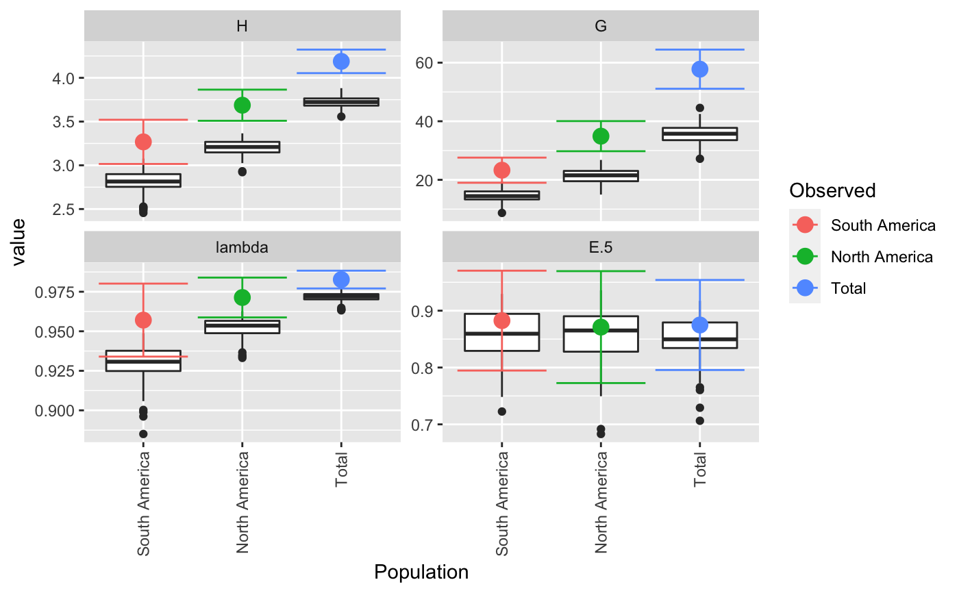
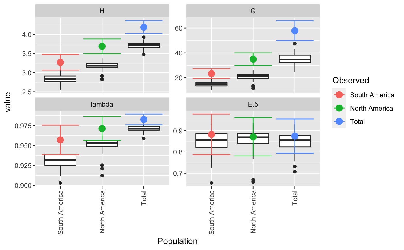
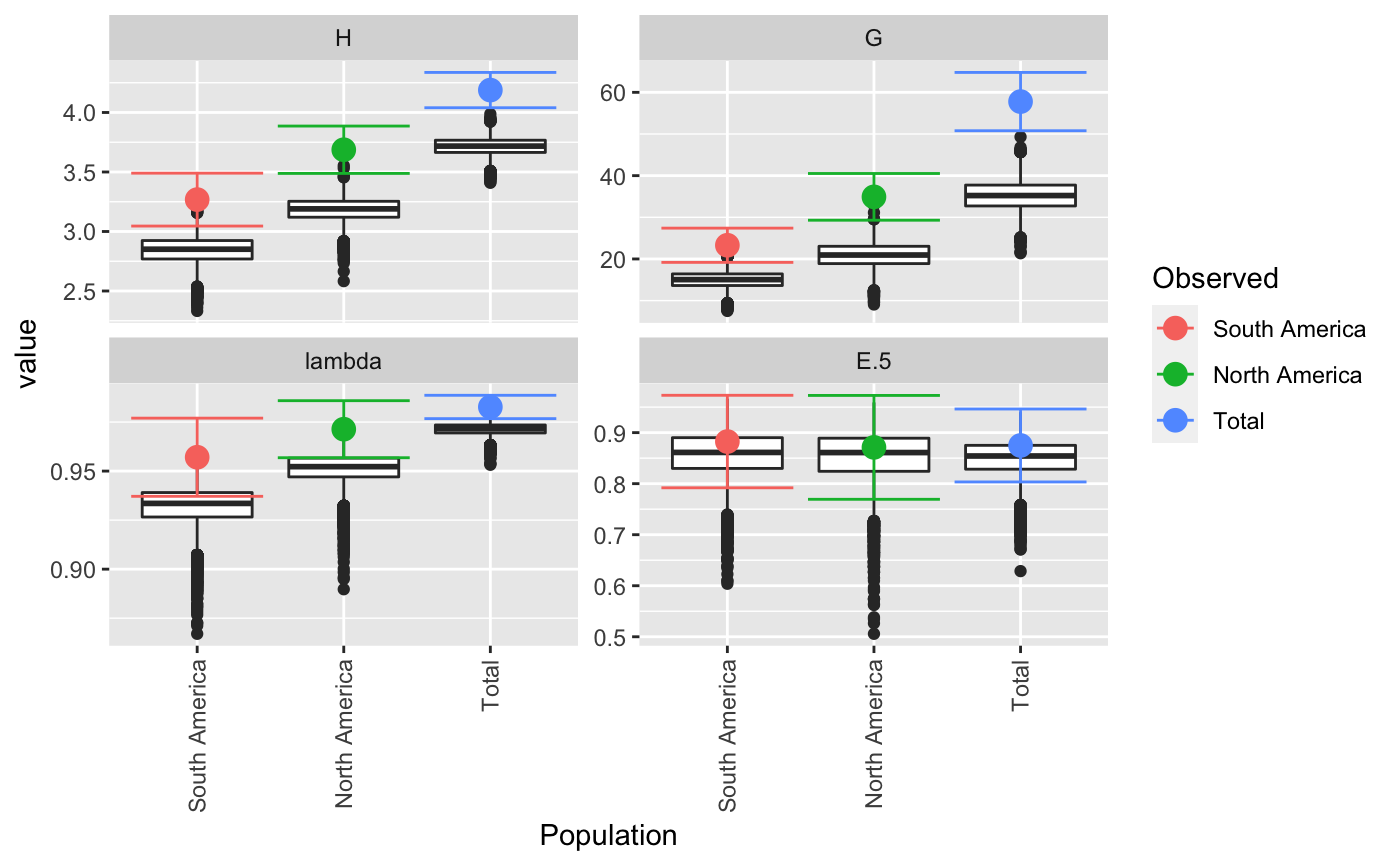
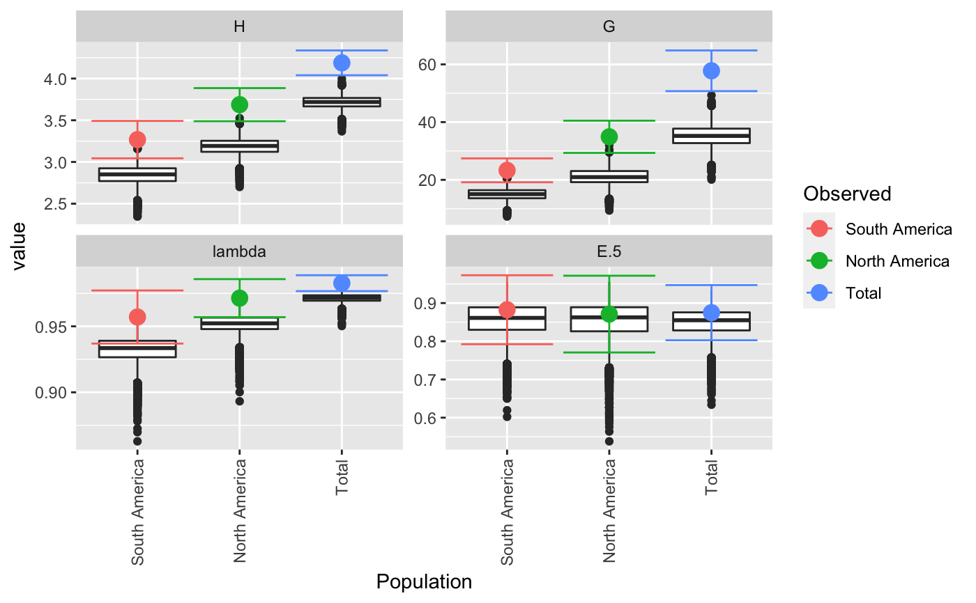
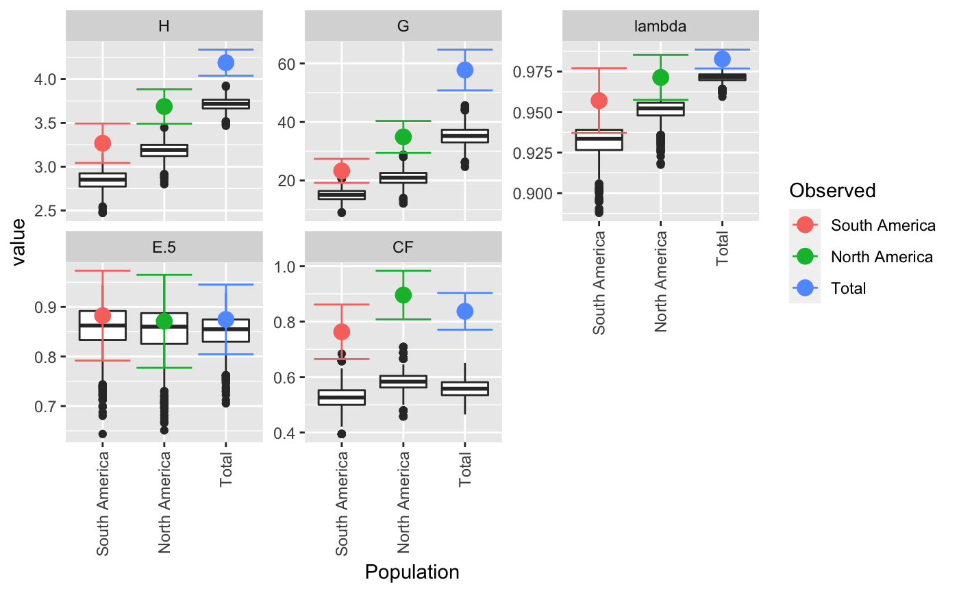
| plot | If `TRUE` (default), boxplots will be produced for each population, grouped by statistic. Colored dots will indicate the observed value.This plot can be retrieved by using `p <- last_plot()` from the ggplot2 package. |
| raw | if `TRUE` (default) a list containing three elements will be returned |
| center | if `TRUE` (default), the confidence interval will be centered around the observed statistic. Otherwise, if `FALSE`, the confidence interval will be bias-corrected normal CI as reported from [boot::boot.ci()] |
| ... | parameters to be passed on to [boot::boot()] and [diversity_stats()] |
Value
raw = TRUE
- **obs** a matrix with observed statistics in columns, populations in rows - **est** a matrix with estimated statistics in columns, populations in rows - **CI** an array of 3 dimensions giving the lower and upper bound, the index measured, and the population. - **boot** a list containing the output of [boot::boot()] for each population.
raw = FALSE
a data frame with the statistic observations, estimates, and confidence intervals in columns, and populations in rows. Note that the confidence intervals are converted to characters and rounded to three decimal places.
Details
Bootstrapping
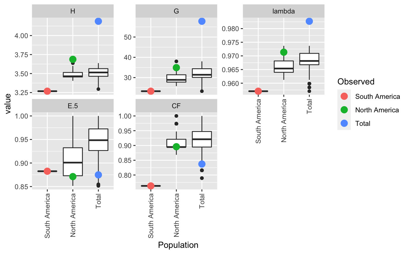
For details on the bootstrapping procedures, see [diversity_boot()]. Default bootstrapping is performed by sampling N samples from a multinomial distribution weighted by the relative multilocus genotype abundance per population where N is equal to the number of samples in the data set. If n.boot > 2, then n.boot samples are taken at each bootstrap replicate. When `rarefy = TRUE`, then samples are taken at the smallest population size without replacement. This will provide confidence intervals for all but the smallest population.
Confidence intervals
Confidence intervals are derived from the function [boot::norm.ci()]. This function will attempt to correct for bias between the observed value and the bootstrapped estimate. When `center = TRUE` (default), the confidence interval is calculated from the bootstrapped distribution and centered around the bias-corrected estimate as prescribed in Marcon (2012). This method can lead to undesirable properties, such as the confidence interval lying outside of the maximum possible value. For rarefaction, the confidence interval is simply determined by calculating the percentiles from the bootstrapped distribution. If you want to calculate your own confidence intervals, you can use the results of the permutations stored in the `$boot` element of the output.
Rarefaction
Rarefaction in the sense of this function is simply sampling a subset of the data at size **n.rare**. The estimates derived from this method have straightforward interpretations and allow you to compare diversity across populations since you are controlling for sample size.
Plotting
Results are plotted as boxplots with point estimates. If there is no rarefaction applied, confidence intervals are displayed around the point estimates. The boxplots represent the actual values from the bootstrapping and will often appear below the estimates and confidence intervals.
Note
Confidence interval calculation
Almost all of the statistics supplied here have a maximum when all genotypes are equally represented. This means that bootstrapping the samples will always be downwardly biased. In many cases, the confidence intervals from the bootstrapped distribution will fall outside of the observed statistic. The reported confidence intervals here are reported by assuming the variance of the bootstrapped distribution is the same as the variance around the observed statistic. As different statistics have different properties, there will not always be one clear method for calculating confidence intervals. A suggestion for correction in Shannon's index is to center the CI around the observed statistic (Marcon, 2012), but there are theoretical limitations to this. For details, see <http://stats.stackexchange.com/q/156235/49413>.
User-defined functions
While it is possible to use custom functions with this, there are three important things to remember when using these functions:
1. The function must return a single value. 2. The function must allow for both matrix and vector inputs 3. The function name cannot match or partially match any arguments from [boot::boot()]
Anonymous functions are okay
(e.g. `function(x)
vegan::rarefy(t(as.matrix(x)), 10)`).
References
Marcon, E., Herault, B., Baraloto, C. and Lang, G. (2012). The Decomposition of Shannon’s Entropy and a Confidence Interval for Beta Diversity. *Oikos* 121(4): 516-522.
See also
[diversity_boot()] [diversity_stats()] [poppr()] [boot::boot()] [boot::norm.ci()] [boot::boot.ci()]
Examples
#> #> #>#> $obs #> Index #> Pop H G lambda E.5 #> South America 3.267944 23.29032 0.9570637 0.8825297 #> North America 3.687013 34.90909 0.9713542 0.8711297 #> Total 4.188215 57.78125 0.9826933 0.8748360 #> #> $est #> Index #> Pop H G lambda E.5 #> South America 2.810714 14.50911 0.9293629 0.8545902 #> North America 3.197910 21.22096 0.9521007 0.8553062 #> Total 3.723559 35.49926 0.9715603 0.8504923 #> #> $CI #> , , Pop = South America #> #> Index #> CI H G lambda E.5 #> 2.5 % 3.015398 18.99547 0.9339777 0.7946645 #> 97.5 % 3.520490 27.58517 0.9801498 0.9703949 #> #> , , Pop = North America #> #> Index #> CI H G lambda E.5 #> 2.5 % 3.508988 29.77002 0.9587624 0.7726727 #> 97.5 % 3.865038 40.04816 0.9839460 0.9695868 #> #> , , Pop = Total #> #> Index #> CI H G lambda E.5 #> 2.5 % 4.053701 51.09567 0.9770752 0.7956329 #> 97.5 % 4.322728 64.46683 0.9883115 0.9540391 #> #> #> $boot #> $boot$`South America` #> #> PARAMETRIC BOOTSTRAP #> #> #> Call: #> boot::boot(data = xi, statistic = boot_stats, R = n, sim = "parametric", #> ran.gen = rg, mle = mle, H = H, G = G, lambda = lambda, E5 = E5) #> #> #> Bootstrap Statistics : #> original bias std. error #> t1* 3.2679442 -0.45723059 0.12885234 #> t2* 23.2903226 -8.78121073 2.19128951 #> t3* 0.9570637 -0.02770083 0.01177882 #> t4* 0.8825297 -0.02793955 0.04483001 #> #> $boot$`North America` #> #> PARAMETRIC BOOTSTRAP #> #> #> Call: #> boot::boot(data = xi, statistic = boot_stats, R = n, sim = "parametric", #> ran.gen = rg, mle = mle, H = H, G = G, lambda = lambda, E5 = E5) #> #> #> Bootstrap Statistics : #> original bias std. error #> t1* 3.6870132 -0.48910283 0.090830659 #> t2* 34.9090909 -13.68813373 2.622024383 #> t3* 0.9713542 -0.01925347 0.006424512 #> t4* 0.8711297 -0.01582350 0.050234108 #> #> $boot$Total #> #> PARAMETRIC BOOTSTRAP #> #> #> Call: #> boot::boot(data = xi, statistic = boot_stats, R = n, sim = "parametric", #> ran.gen = rg, mle = mle, H = H, G = G, lambda = lambda, E5 = E5) #> #> #> Bootstrap Statistics : #> original bias std. error #> t1* 4.1882146 -0.46465576 0.068630576 #> t2* 57.7812500 -22.28198749 3.411071183 #> t3* 0.9826933 -0.01113304 0.002866475 #> t4* 0.8748360 -0.02434370 0.040410486 #> #># \dontrun{ # With pretty results diversity_ci(Pinf, n = 100L, raw = FALSE)#> #> #>#> H H.est H.ci G G.est G.ci lambda #> South America 3.27 2.84 (3.065, 3.471) 23.3 14.8 (19.394, 27.186) 0.957 #> North America 3.69 3.18 (3.492, 3.882) 34.9 20.9 (29.778, 40.04) 0.971 #> Total 4.19 3.71 (4.024, 4.353) 57.8 35.0 (49.827, 65.736) 0.983 #> lambda.est lambda.ci E.5 E.5.est E.5.ci #> South America 0.931 (0.938, 0.976) 0.883 0.851 (0.787, 0.978) #> North America 0.951 (0.956, 0.986) 0.871 0.857 (0.781, 0.961) #> Total 0.971 (0.976, 0.989) 0.875 0.849 (0.794, 0.955)# This can be done in a parallel fasion (OSX uses "multicore", Windows uses "snow") system.time(diversity_ci(Pinf, 10000L, parallel = "multicore", ncpus = 4L))#> #> #>#> user system elapsed #> 10.103 3.262 4.297#> #> #>#> user system elapsed #> 7.400 0.153 7.569# We often get many requests for a clonal fraction statistic. As this is # simply the number of observed MLGs over the number of samples, we # recommended that people calculate it themselves. With this function, you # can add it in: CF <- function(x){ x <- drop(as.matrix(x)) if (length(dim(x)) > 1){ res <- rowSums(x > 0)/rowSums(x) } else { res <- sum(x > 0)/sum(x) } return(res) } # Show pretty results diversity_ci(Pinf, 1000L, CF = CF, center = TRUE, raw = FALSE)#> #> #>#> H H.est H.ci G G.est G.ci lambda #> South America 3.27 2.84 (3.043, 3.493) 23.3 15.0 (19.182, 27.399) 0.957 #> North America 3.69 3.18 (3.49, 3.884) 34.9 20.9 (29.449, 40.37) 0.971 #> Total 4.19 3.71 (4.039, 4.337) 57.8 35.2 (50.814, 64.748) 0.983 #> lambda.est lambda.ci E.5 E.5.est E.5.ci CF #> South America 0.932 (0.937, 0.977) 0.883 0.856 (0.792, 0.973) 0.763 #> North America 0.951 (0.958, 0.985) 0.871 0.852 (0.777, 0.965) 0.896 #> Total 0.971 (0.977, 0.989) 0.875 0.850 (0.804, 0.945) 0.837 #> CF.est CF.ci #> South America 0.528 (0.665, 0.862) #> North America 0.583 (0.808, 0.984) #> Total 0.558 (0.771, 0.903)diversity_ci(Pinf, 1000L, CF = CF, rarefy = TRUE, raw = FALSE)#> #>#> H H.est H.ci G G.est G.ci lambda #> South America 3.27 3.27 <NA> 23.3 23.3 <NA> 0.957 #> North America 3.69 3.48 (3.405, 3.565) 34.9 29.5 (25.786, 34.381) 0.971 #> Total 4.19 3.50 (3.355, 3.601) 57.8 31.5 (25.786, 36.1) 0.983 #> lambda.est lambda.ci E.5 E.5.est E.5.ci CF #> South America 0.957 <NA> 0.883 0.883 <NA> 0.763 #> North America 0.966 (0.961, 0.971) 0.871 0.904 (0.851, 0.972) 0.896 #> Total 0.968 (0.961, 0.972) 0.875 0.944 (0.873, 0.985) 0.837 #> CF.est CF.ci #> South America 0.763 <NA> #> North America 0.906 (0.868, 0.947) #> Total 0.909 (0.816, 0.974)# }