Chapter 4 Spatial and Temporal Analysis of Populations of the Sudden Oak Death Pathogen in Oregon Forests

Zhian N. Kamvar, Meredeth M. Larsen, Alan M. Kanaskie, Everett M. Hansen, and Niklaus J. Grünwald

Journal: Phytopathology

3340 Pilot Knob Rd, St Paul, MN 55121, USA

Published 2015-07, Volume 105, Issue: 7, DOI: 10.1094/PHYTO-12-14-0350-FI

4.1 Abstract

Sudden oak death caused by the oomycete Phytophthora ramorum was first discovered in California toward the end of the 20th century and subsequently emerged on tanoak forests in Oregon before its first detection in 2001 by aerial surveys. The Oregon Department of Forestry has since monitored the epidemic and sampled symptomatic tanoak trees from 2001 to the present. Populations sampled over this period were genotyped using microsatellites and studied to infer the population genetic history. To date, only the NA1 clonal lineage is established in this region, although three lineages exist on the North American west coast. The original introduction into the Joe Hall area eventually spread to several regions: mostly north but also east and southwest. A new introduction into Hunter Creek appears to correspond to a second introduction not clustering with the early introduction. Our data are best explained by both introductions originating from nursery populations in California or Oregon and resulting from two distinct introduction events. Continued vigilance and eradication of nursery populations of P. ramorum are important to avoid further emergence and potential introduction of other clonal lineages.

4.2 Introduction

Sudden oak death (SOD) emerged as a severe epidemic disease on coast live oak (Quercus agrifolia) and tanoak (Notholithocarpus densiflorus) in California in the mid 1990s and reemerged shortly thereafter on tanoak in Oregon in the early 2000s (Everhart et al., 2014; Grünwald et al., 2008a; Hansen et al., 2008; Rizzo et al., 2005). SOD is caused by Phytophthora ramorum Werres, De Cock & Man in’t Veld, and is considered to be one of the top two oomycete pathogens based on its scientific and economic importance (Kamoun et al., 2014; Werres et al., 2001). The Oregon epidemic was first detected during aerial surveys in 2001 on tanoak but likely derived from initial introductions in the late 1990s. The Oregon Department of Forestry has since monitored the epidemic and sampled symptomatic tanoaks since 2001 (Hansen et al., 2008). Strains sampled from infected sites in forest or nursery environments have been genotyped in several labs using a range of microsatellite loci (Grünwald et al., 2009; Ivors et al., 2006; Prospero et al., 2004, 2009, 2007).

P. ramorum has emerged repeatedly around the world as 4 distinct clonal lineages found in North America (lineages NA1, NA2, and EU1) and Europe (EU1 and EU2) (Grünwald et al., 2012; Ivors et al., 2006; Poucke et al., 2012). The lineages have been named by the continent on which they first appeared, i.e. North America (= NA) or Europe (= EU) and are numbered in order of discovery (Grünwald et al., 2009). The NA1 clonal lineage was first discovered in California causing SOD on tanoak and coast live oak and is the one currently found in Curry County, Oregon, USA (Mascheretti et al., 2008). The EU1 and NA2 populations were discovered later in nursery environments and are currently only found in California, Oregon, Washington and British Columbia while the NA1 clone has been shipped with nursery plants from the West to the Southern and Southwestern US (Goss et al., 2009, 2011; Grünwald et al., 2012; Ivors et al., 2006; Mascheretti et al., 2008; Prospero et al., 2009). The EU1 clonal lineage is the one first discovered in Europe, but in 2007 the new EU2 lineage emerged in Northern Ireland and since migrated to Western Scotland (Poucke et al., 2012; Werres et al., 2001). EU1 was first introduced to Europe and eventually migrated to the Pacific Northwest of North America (Goss et al., 2011).

P. ramorum populations sampled in Oregon forests to date belong exclusively to the NA1 clonal lineage (Hansen et al., 2008; Prospero et al., 2007). Given that NA2 and/or EU1 clones have been found in California, Oregon, Washington, and/or British Columbia in association with nursery plant movements, introduction of NA2 or EU1 from nursery environments to Curry County forests is a plausible scenario (Goss et al., 2009, 2011; Grünwald et al., 2012; Prospero et al., 2009, 2007). Our present work thus monitors populations and potential emergence of novel lineages in Oregon forests.

Our main objectives here are to describe the spatial and temporal pattern of the populations and clonal dynamic of the SOD pathogen in Curry County in southwestern Oregon from 2001 to the present. Specifically, we asked (1) if novel lineages have been introduced into the forests in Curry County, (2) if multiple introductions occurred, and (3) whether introduction might have come from nursery populations. We sampled infected tanoaks between 2001-2014 and characterized populations using microsatellite analysis.

4.3 Materials and Methods

4.3.1 Location

The SOD infested areas are located in the Siskiyou Mountains of Curry County in south western Oregon near the town of Brookings (42.0575\(^{\circ}\) N, 124.2864\(^{\circ}\) W) on the coast (Figure 4.1) (Prospero et al., 2007). The Siskiyou mountains form part of the Klamath Mountain range (Franklin and Dyrness 1988). The vegetation in SOD infested areas is a mosaic of different vegetation types including mixed-evergreen, redwood (Sequoia sempervirens) and Douglas-fir (Pseudotsuga menziesii) forests with tanoak as the dominant SOD host.

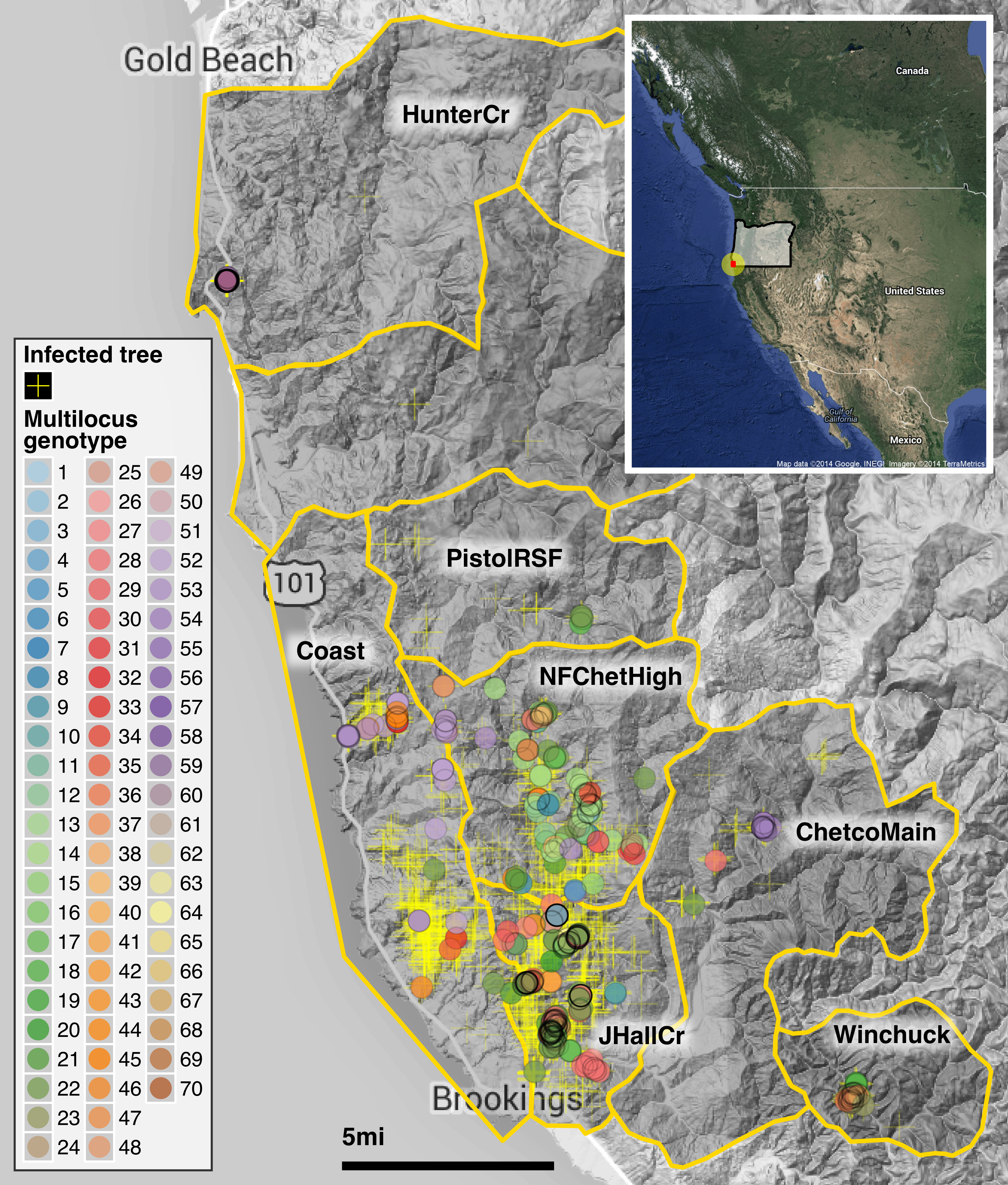
Figure 4.1: Spatial distribution of the SOD epidemic and multilocus genotypes of Phytophthora ramorum in Curry County, Oregon. The yellow crosses mark tanoak trees found positive for P. ramorum during aerial surveys. A total of 70 multilocus genotypes have been identified between 2001-2014 and are marked by color as shown in the legend. The abbreviations for regions shown in the map are explained in Table 4.1. The inset shows the placement of Curry county (red dot) in SW Oregon.

4.3.2 Sampling

Commencing in 2001, 2-4 aerial surveys per year were conducted over the tanoak range by the Oregon Department of Forestry and the USDA Forest Service in Curry County. The survey detects recently killed tanoaks based on the reddish-brown color of foliage (Hansen et al., 2008). All trees identified by aerial surveys were ground checked and geographically referenced using a hand-held GPS instrument (Garmin GPS 12XL or 60CX, Garmin International, Olathe, KS). Bark or foliage samples were collected for determination of P. ramorum presence by culturing in the field and laboratory. Host plants within the area of the delimitation survey, generally 300 feet, were also inspected and sampled if they were symptomatic. Maps of distribution were prepared using ArcView GIS version 3.3 and ArcMap version 10.2 (Environmental Systems Research Institute, Redlands, CA).

4.3.3 Isolation, identification and DNA extraction

Table 4.1: Summary of P. ramorum isolates sampled in Oregon forests and multilocus genotypes (MLG)observed across regions and years.

Abbreviation	Region name	Year	Number of isolates	MLGs detected (region specific)
JHallCr	Joe Hall Creek	2001, 2002, 2003, 2004, 2005, 2013, 2014	244	30 (19)
NFChetHigh	North Fork Chetco	2003, 2012, 2013, 2014	114	35 (19)
Coast	Coastal Region	2006, 2010, 2011, 2012, 2013, 2014	34	12 (7)
HunterCr	Hunter Creek; Cape Sebastian	2011	66	4 (4)
Winchuck		2012, 2013	35	9 (3)
ChetcoMain		2013, 2014	16	7 (1)
PistolRSF	Pistol River South Fork	2013	4	2 (0)
Total	-	2001-2014	513	70 (53)

Isolations were made from symptomatic plant tissue onto selective CARP agar (Difco corn meal agar, 10 ppm natamycin, 200pm NA-ampicillin, and 10 ppm rifampicin) (Prospero et al., 2007). Candidate Phytophthora cultures were transferred onto corn meal agar with 30 ppm \(\beta\)-sitosterol. P. ramorum identification was confirmed by microscopic inspection for presence of characteristic chlamydospores and deciduous sporangia (Werres et al., 2001). Genomic DNA was extracted using either the FastDNA SPIN kit (MP Biomedicals, LLC; 116540600) (Goss et al., 2009) or the cetyltrimethyl ammonium bromide (CTAB )-chloroform-isopropanol method (Winton & Hansen, 2001). Table 4.1 provides an overview of strains collected by year and region following regions as shown in figure 4.1.

4.3.4 Genotyping, data validation, and harmonization

Five microsatellite loci were utilized in this analysis: PrMS6, Pr9C3, PrMS39, PrMS45, and PrMS43 (Grünwald et al., 2009, 2008b; Prospero et al., 2004, 2007). Genotyping (see specific protocols in supplementary text) of P. ramorum strains collected 2001-2012 occurred over several years and in several laboratories, with different protocols and sequencers. Consequently, a concerted effort was made to create a comprehensive dataset with identical allele calls. To detect errors, allele calls from all five genotyped loci were generated for a subsample of 40 isolates representing the most common multilocus genotypes from the culture collection, and then compared to data from participating laboratories. Three of the five loci, PrMS6, Pr9C3, and PrMS39 had identical allele calls between laboratories for the subsampled isolates. The remaining two loci, PrMS45 and PrMS43, had allele calls that differed by a single bp between laboratories. Data from PrMS45 and PrMS43 were therefore corrected to allow consistent comparisons of allele calls. Given the varied nature of the genotyping data described above genotyping of P. ramorum strains consists of two datasets including either 5 loci (2001-14) or a newly developed, multiplexed method including 14 loci (samples 2013-14) (Table 4.2). Details on both genotyping methods can be found in the supplementary text 4.7.1 and figure 4.6.

Table 4.2: Newly multiplexed protocol for P. ramorum primer sequences of simple sequence repeat (SSR) loci and final concentrations used to determine multilocus genotypes for four clonal lineages. PrMS6, Pr9C3, PrMS39, PrMS45, and PrMS43 were utilized in this study as they were commonly genotyped across all laboratories.

SSR Locus	Dye	Product (bp)c	Primer sequenceb	Final conc. (µM)	Reaction
ILVOPrMS145abcf	6-FAM	167-257	Fwd6FAM-TGGCAGTGTTCTTCAACAGC Rev-GTTTATTCCCGTGAACAGCGTATC	0.04	8-plex
PrMS39d	NED	130-258	FwdNED-GCACGGCCAGAGATTGATAG Rev-GTTTATCTGCCGACGTGAAGAAGT	0.07	8-plex
PrMS9C3d	PET	210-226	FwdVIC-TCACACGAAGCAGCAACTCT Rev-GTTTAGCGGCACTACGGAATACAT	0.04	8-plex
ILVOPrMS79af	6-FAM	342-396	Fwd6FAM-AGGCGGAAAACGTCAGAAC Rev-GTTTCTCGAGAGGCTGGAAGTACG	0.15	8-plex
KI18e	VIC	217-279	FwdPET-TGCCATCACAACACAAATCC Rev-GTTTGTGCTATCTTTCCTGAACGG	1.0	8-plex
KI64e	NED	342-401	FwdNED-GCGCTAAGAAAGACACTCCG Rev-GTTTCAACATGTAGCCATTGCAGG	0.35	8-plex
PrMS45d	VIC	138-186	FwdVIC-CGTGCTGCATCTGGTGTAGT Rev-GAAAGTCCGGATTTGCGTTA	0.15	8-plex
PrMS6d	PET	165-168	FwdPET-AATCGATCTCTCGGCTTTGA Rev-TATAGCCCCAGCTGCAACA	0.15	8-plex
ILVOPrMS131f	VIC	146-414	FwdVIC-CGGCCGTTTTTGTAAGTTTG Rev-GTTTCAGATCAAACCAAAATCTGCTC	0.2	2-plex
KI82abe	NED	95-243	FwdNED-CCACGTCATTGGGTGACTTC Rev-GTTTCGTACAAGTCACGACTCCCC	0.2	2-plex
PrMS43d	6-FAM	122-493	Fwd6FAM-AAATATGCAAAAAGGCAGGA Rev-GTTTCCGCGTAACCTAGTCTGCTC	0.3	Simplex

^a ILVOPrMS79 amplifies three alleles in the NA1 lineage. The first two alleles are fixed and the third is polymorphic.
^b Reverse (Rev) primer includes PIG tail addition except for PrMS45 and PrMS6. Indicated in italic.
^c Product size range is for four lineages (EU1, EU2, NA1, NA2). Only the NA1 lineage has been reported in Curry County,OR forests.
^d Described by Prospero et al. (2004) and/or Prospero et al. (2007).
^e Described by Ivors et al. (2006).
^f Described by Vercauteren et al. (2010), and Vercauteren et al. (2011).

4.3.5 Nursery populations

To determine if forest populations cluster with different nursery populations from Oregon or California, we used previously published data from our work to determine relationships among nursery and Curry County forest populations (Goss et al., 2009, 2011; Grünwald et al., 2009; Prospero et al., 2009, 2007).

4.3.6 Data analysis

All individuals genotyped for this effort belonged to the NA1 clonal lineage (Grünwald et al., 2009). Thus, all analyses presented here focused on describing the clonal dynamic using model-free approaches that avoid violation of population genetic theory. Samples were grouped into different multilocus genotypes (MLGs) defined by the unique combination of alleles across all observed loci from the consensus five SSR loci genotyped across all years. For identification purposes, unique MLGs were then assigned an arbitrary number from 1 to the total number of observed MLGs. Population genetic analysis was conducted using the computer and statistical language R (R Core Team, 2014) using various packages as well as R functions written specifically for this project (see github link below). Graphs and figures were created using the R packages ggplot2, ape, igraph, ggmap, and poppr (Csardi & Nepusz, 2006; Kahle & Wickham, 2013; Kamvar et al., 2014b; Paradis et al., 2004; Wickham, 2009). Within-locus allelic diversity was analyzed across and within years and regions using the function locus_table() from the R package poppr (Table 4.5) (Kamvar et al., 2014b). To address the temporal and spatial aspects of the data, populations were analyzed both by year isolated and watershed region (Table 4.1; Fig. 4.1). Watershed regions were drawn with ArcMap version 10.2 (Environmental Systems Research Institute, Redlands, CA). The regions represent drainages or portions of drainages in which infected trees were discovered as the disease progressed over time. In most cases, ridgelines dividing drainages formed the boundary of a region. These regions were saved as shapefiles and imported into R with rgdal (Bivand et al., 2014).

Genotypic diversity was analyzed within and across years and populations, with the Shannon-Wiener index (H) and the Stoddard and Taylor’s index (G), (Shannon, 1948; Stoddart & Taylor, 1988). Both G and H measure genotypic diversity, combining richness and evenness. If all genotypes are equally abundant, then the value of G will be the number of MLGs and the value of H will be the natural log of the number of MLGs. Both G and H are used as they weigh more or less abundant MLGs more heavily, respectively (Grünwald et al., 2003). Evenness was calculated as E₅, which is an estimator of evenness that utilizes both H and G that gives a ratio of the number of abundant genotypes to rare genotypes (Grünwald et al., 2003; Ludwig & Reynolds, 1988; Pielou, 1975). These were calculated with the R packages poppr and vegan (Kamvar et al., 2014b; Oksanen et al., 2013). Confidence intervals were calculated using the R package boot with 9,999 bootstrap resamplings (Canty & Ripley, 2015). Richness, or the expected number of MLGs (eMLG), was calculated using rarefaction from the R packages poppr and vegan (Heck et al., 1975; Hurlbert, 1971). Some statistics (AMOVA, genotypic diversity, index of association, allelic diversity, and Nei’s distance) were also performed on clone-censored data where each MLG was represented once per population hierarchy.

Because the analysis of genotypic diversity, richness and evenness is agnostic to specific alleles within MLGs, assessment of genetic relatedness between MLGs was performed using the function bruvo.dist() using poppr, which calculates Bruvo’s genetic distance, utilizing a stepwise mutation model for microsatellite loci (Bruvo et al., 2004; Kamvar et al., 2014b). This distance thus gives a more fine-scale picture of relationships between individuals than band-sharing models. These relationships were visualized with minimum spanning networks generated using the R packages igraph and poppr (Csardi & Nepusz, 2006; Kamvar et al., 2014b).

If the epidemic had a single origin, a correlation between genetic and geographic distance would be expected as populations acquire mutations over time and clonally diverge regardless of rates of spread. This was tested by performing Mantel tests across all hierarchical levels in the data set utilizing the function mantel.randtest() in the R package ade4 between Bruvo’s distance as described above and Euclidean distances between geographic coordinates (Dray & Dufour, 2007; Mantel, 1967). P-values were calculated using 99,999 bootstrap replicates.

As the eradication efforts destroy the immediate habitat in an infected area, one question that we wanted to address was whether or not genotypes were clustering to specific regions or if they were evenly spread throughout Curry County (Prospero et al., 2007). This was tested using three methods: bootstrap analysis of Nei’s genetic distance, Analysis of MOlecular VAriance (AMOVA), and Discriminant Analysis of Principal Components (DAPC) in the R packages poppr, ade4, and adegenet (Excoffier et al., 1992; Jombart et al., 2010; Kamvar et al., 2014b). The bootstrap analysis utilized 10,000 bootstrap replicates treating loci as independent units with the function aboot() in poppr and was visualized as an unrooted neighbor-joining tree in figtree v. 1.4.2 (Figure 4.5). AMOVA utilizes a distance matrix between genotypes for which hierarchical partitions are defined and attempts to analyze the variation within samples, between samples, between subpopulations within populations and finally between populations. In this case, we used both the hierarchies of samples within years within regions and samples within regions within years. DAPC is a multivariate, model-free approach to clustering based on prior population information (Jombart et al., 2010). This allows us to analyze the population structure by assessing how well samples can be reassigned into previously defined populations. Both DAPC and AMOVA were run with and without Hunter Creek and Pistol River South Fork due to isolated genotypes and small sample size, respectively. For the DAPC analysis, these removed populations had their origins predicted from the DAPC object using the function predict.dapc in the R package adegenet (Jombart et al., 2010).

Since DAPC is sensitive to the number of principal components used in analysis, the function xvalDapc() from the R package adegenet was used to select the correct number of principal components with 1,000 replicates using a training set of 90% of the data. The number of principal components was chosen based on the criteria that it had to produce the highest average percent of successful reassignment and lowest root mean squared error (Jombart et al., 2010). Significant deviations from random population structure was tested in AMOVA utilizing the function randtest() from the R package ade4 with 9,999 bootstrap replicates (Dray & Dufour, 2007).

All data and R scripts to reproduce the analyses shown here are deposited publicly on github (https://github.com/grunwaldlab/Sudden_Oak_Death_in_Oregon_Forests) and citable (DOI: 10.5281/zenodo.13007).

4.4 Results

4.4.1 Demographic pattern and genetic diversity

The epidemic has expanded over time from the initial focus in Joe Hall Creek NE of Brookings, Oregon mostly north (first to N Fork Chetco High) and northwest (Coast, Pistol River South Fork), but also east (Chetco Main and Winchuck) (Fig. 4.1; Table 4.1). To date a total of 70 multilocus genotypes have been found in forest populations (Table 4.1). MLG 22 is most abundant and the only MLG detected across the whole period (although it was not sampled in every year) (Fig. 4.2). MLG 59, the second most abundant MLG, was only detected in 2011 and has a high frequency due to the sampling design applied: all 2011 strains were sampled in one concentrated area in the northwestern sampling range geographically distant from any other location (Fig. 4.2). Given that sampling strategies for some years were not comprehensive, samples from some years have to be interpreted with caution (e.g., 2005-6, 2010-11). Samples from 2013 and 2014 are sampled from all regions and can be considered more representative.

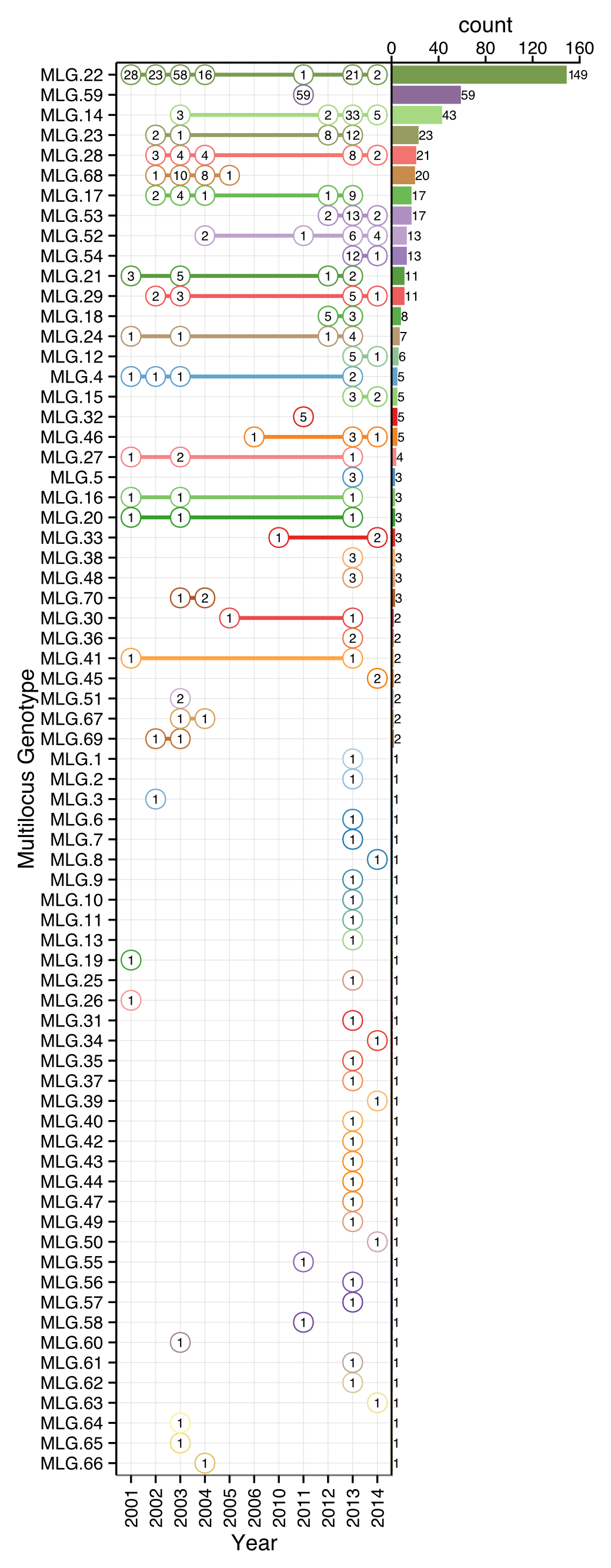
Figure 4.2: Rank distribution of multilocus genotypes (MLGs) of P. ramorum and recovery per year. The vertical axis denotes unique MLGs detected in the whole data set with decreasing abundance as indicated by the barplot on the right side. The horizontal axis indicates year of sampling. Each numbered circle represents the number of observations of each MLG with lines connecting genotypes found in multiple years.

Allelic and genotype diversity within loci revealed that PrMS43 had, on average, the highest number of alleles (n = 18). All other loci had 5 or fewer alleles with a moderate to high amount of diversity (Table 4.6). Nevertheless, the genotype accumulation curve showed a slight plateau, indicating that we have enough power in our data to describe a significant number of MLGs (Fig. 4.7). Genotypic diversity (H = 2.98, G = 8.64), evenness (E₅ = 0.41), and richness (eMLG = 7) were low as expected for a clonal population slowly accumulating mutations over space and time (Table 4.7). A pattern of increasing diversity across years (with number of MLGs not fewer than 10) was also observed (Table 4.7). The minimum spanning network showed that MLGs 17, 22, and 28 clustered in the center of the network and had the highest number of connections to other genotypes in the forest populations (Fig. 4.3). Most genotypes were connected to their immediate neighbors by a genetic distance of 0.05 or the equivalent of one mutational step across 5 diploid loci.

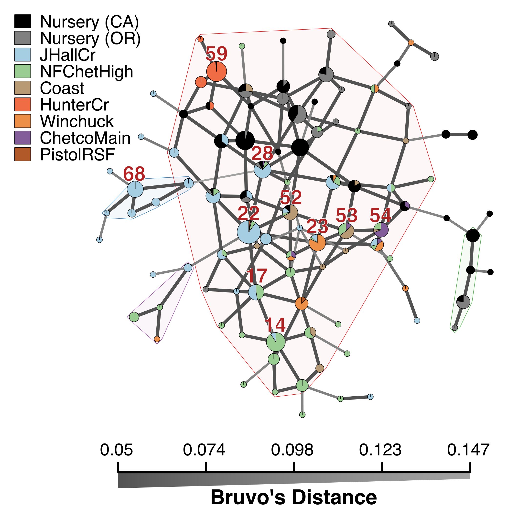
Figure 4.3: Minimum spanning network based on Bruvo’s genetic distance for microsatellite markers for P. ramorum populations. Nodes (circles) represent individual multilocus genotypes. The 10 most abundant forest genotypes are labeled with their MLG designation. Node colors represent population membership proportional to the pie size. Node sizes are relatively scaled to log_1.75n, where n is the number of samples in the nodes to avoid node overlap. Edges (lines) represent minimum genetic distance between individuals determined by Prim’s algorithm. Nodes that are more closely related will have darker and thicker edges whereas nodes more distantly related will have lighter and thinner edges or no edge at all. Reticulation was introduced by finding exact ties in genetic distance after Prim’s algorithm was run. Subgroups of >3 MLGs where all nodes are no more than one mutational step (d = 0.05) away from its neighbors, are highlighted in arbitrary colors.

4.4.2 Spatial Correlation

A Mantel test revealed significant correlations of genetic distance and geographic distance for most samples collected after 2003 (Table 4.3). When partitioned by year, this correlation appears to increase and become more pronounced with the progression of the epidemic. When partitioned by region, those that are closer to the origin of the epidemic (Joe Hall Creek and N Fork Chetco River) show significant correlation. When the overall mantel test was run without Hunter Creek, the correlation coefficient was reduced (0.175), but was still significant (p = 0.0001).

Table 4.3: Table of correlation coefficients generated across forest regions and years of P. ramorum isolates using the Mantel test. Euclidean distances were calculated from geographic coordinates while genetic distance was based on Bruvo’s distance. Significance of values are based on 99,999 Monte-Carlo permutations and marked as follows: * ≤ 0.05, ** ≤ 0.01, *** ≤ 0.001, - = no data, NaN = insufficient data for analysis.

	2001	2002	2003	2004	2005	2006	2010	2011	2012	2013	2014	Pooled
JHallCr	0.06	0.24	0.14***	0.28***	NaN	-	-	-	-	0.18**	NaN	0.14***
NFChetHigh	-	-	NaN	-	-	-	-	-	0.68	0.41***	-0.23	0.35***
Coast	-	-	-	-	-	NaN	NaN	NaN	NaN	0.55*	-0.25	0.13
HunterCr	-	-	-	-	-	-	-	0.06	-	-	-	0.06
Winchuck	-	-	-	-	-	-	-	-	0.41**	0.03	-	0.11
ChetcoMain	-	-	-	-	-	-	-	-	-	0.53	NaN	0.63*
PistolRSF	-	-	-	-	-	-	-	-	-	0.94	-	0.94
Pooled	0.06	0.24	0.13***	0.28***	NaN	NaN	NaN	0.87***	0.59***	0.15***	0.14*	0.52***

4.4.3 Population differentiation

Cluster analysis of populations with respect to year using Nei’s genetic distance showed no significant (>70%) bootstrap support for any clades, but does show that these tend to cluster by region as opposed to year (Fig. 4.8). AMOVA analysis revealed significant population structure between regions on both clone-corrected (with respect to hierarchy) and uncorrected data sets (Table ??). Significant structure was only found between years within regions on the uncorrected data set. Both patterns were observed without Hunter Creek and Pistol River South Fork isolates. DAPC clustering showed that the first discriminant component separated Hunter Creek from all other regions and the second discriminant component shows a gradient from Joe Hall Creek to the coast (Fig. 4.4). This distinction was reflected in the percent of correct posterior assignment of isolates to their original populations. Over the whole data set there was an 81.5% assignment- success rate. Hunter Creek received 100% successful reassignment. Joe Hall Creek, Winchuck, and Coast all had >85% successful reassignment whereas Chetco Main, North Fork of the Chetco, and Pistol River South Fork all had <69% successful reassignment (Fig. 4.9). The isolation of the Hunter Creek isolates in the DAPC analysis was found to be mainly driven by allele 493 at locus PrMS43 (Fig. 4.10). The only other population to share this allele was Joe Hall Creek where it was present in a total of 4 isolates, and only isolates found in the coastal region or North Fork Chetco contained the allele 489, which is one mutational step away in a stepwise mutation model of a tetranucleotide repeat locus. When DAPC was run without Hunter Creek and Pistol River South Fork data, percent successful reassignment for all regions did not change significantly. Prediction of sources for the Hunter Creek data revealed that over 98% of the genotypes were assigned to the Coast with a 99% probability.

Table 4.4: AMOVA table generated comparing P. ramorum isolates for two different hierarchies, year within region and region within year, respectively. Results are rounded to three significant figures. Clone corrected results are provided in parentheses. P values are based on 9,999 permutations.

Heirarchy	df	Sum of squares	Variation (%)	P	\(\phi\) statistic
Region by year
Between region	10 (10)	160 (21)	11.6 (3)	0.366 (0.175)	0.448 (0.101)
Between year within region	12 (12)	59.5 (19.1)	33.3 (7.07)	1e-04 (2e-04)	0.376 (0.0729)
Within year within region	490 (129)	281 (141)	55.2 (89.9)	1e-04 (1e-04)	0.116 (0.03)
Year by region
Between year	6 (6)	197 (23)	45 (12.3)	1e-04 (1e-04)	0.496 (0.12)
Between region within year	16 (16)	22.5 (17.2)	4.56 (-0.283)	1e-04 (0.446)	0.0829 (-0.00323)
Within region within year	490 (129)	281 (141)	50.4 (88)	1e-04 (1e-04)	0.45 (0.123)

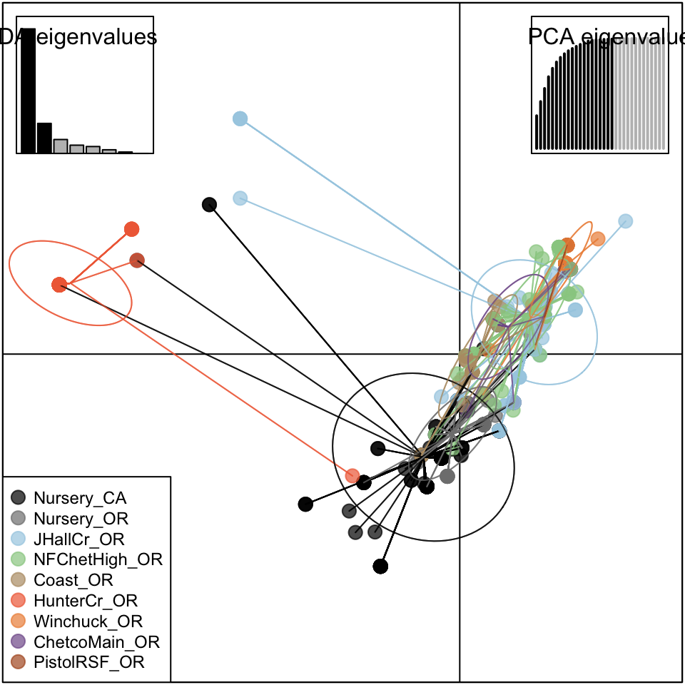
Figure 4.4: Scatterplot from DAPC of the first two principal components discriminating P. ramorum populations by regions. Points represent individual observations. Colors and lines represent population membership. Inertia ellipses represent an analog of a 67% confidence interval based on a bivariate normal distribution.

4.4.4 Clustering of forest with nursery populations

We used previously published data to determine if nursery populations in California or Oregon could have been source populations for the Oregon forest epidemic (Goss et al., 2009, 2011; Grünwald et al., 2009; Prospero et al., 2009, 2007). Nursery data included 40 MLGs across 216 samples of NA1 clones. Of these 40, 12 MLGs matched the forest sample and 28 MLGs were unique to the nurseries. The only region that did not contain genotypes that matched those found in nurseries was Pistol River South Fork. When considering those 12 genotypes that were present in both data sets, with the exception of Joe Hall Creek, all genotypes were first isolated from nurseries before discovery in the forest. At the most variable locus, PrMS43, both nursery populations had the allele 281 at frequencies of 4.5% and 4.9% for CA and OR, respectively. This allele was not observed in the forest population. Both populations contained allele 489 at >10% frequency and the CA nursery population contained allele 493 at a frequency of 1.4%.

When nursery genotypes were added to the minimum spanning network, MLGs found at Hunter Creek, previously isolated in the network, connected by only a single MLG from the coast, gained more connections to nursery MLGs. Clustering with Nei’s distance revealed the Nursery isolates from CA consistently clustering closest with Hunter Creek isolates in both clone-corrected and uncorrected data sets (Fig. 4.5). DAPC clustering revealed a decrease in overall assignment-success rate at 78%. The nursery isolates received 74% and 83% assignment success for CA and OR nurseries, respectively.

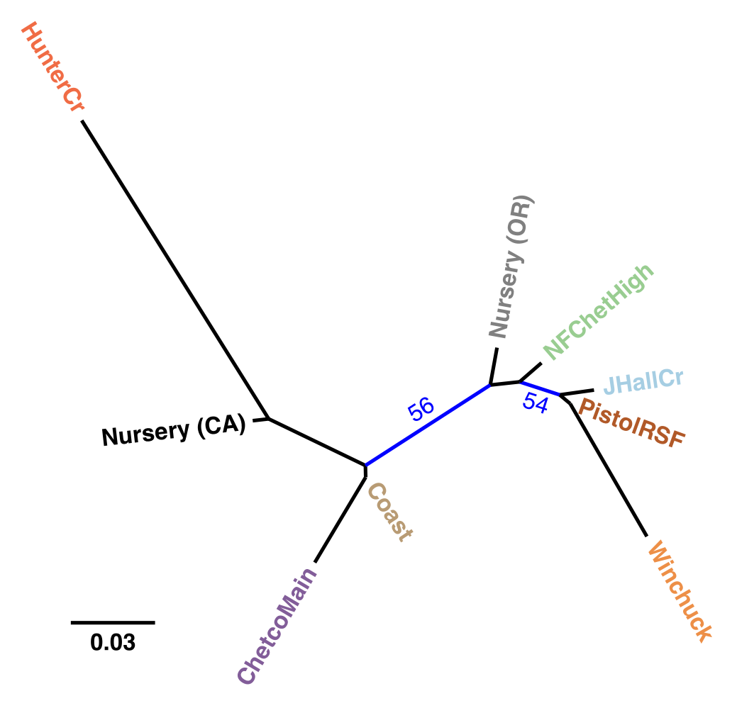
Figure 4.5: Unrooted, neighbor-joining tree with 10,000 bootstrap replicates of Nei’s genetic distance for P. ramorum populations defined by region. Tip labels are colored by region. Branches with bootstrap values greater than 50% are shown in blue. Nursery populations are shown as originating from California (CA) or Oregon (OR).

The assignment successes for the regions before or after inclusion of nursery data changed less than 5% for all regions except for the coast, which saw a decrease of 17.6% when nursery populations were included (Fig. 4.9). Prediction of sources for nursery genotypes against the forest data revealed that 48% of these nursery isolates were predicted to share membership with the coast at \(\geq\) 95% probability (Fig. 4.11, 4.12). A total of 3.2% of the isolates were predicted to share membership with Hunter Creek at \(\geq\) 99.9% membership probability. Furthermore, 21.75% of the nursery data could not be assigned to any of the forest populations at >60% probability.

Since 3.2% of the nursery isolates had a very strong signal for Hunter Creek, we predicted sources for Hunter Creek isolates when considering nursery isolates. This approach determines if Hunter Creek isolates cluster more readily with nursery or coast populations. Indeed, 92% of the Hunter Creek isolates were predicted to share membership with California nurseries at \(\geq\) 99% membership probability (Fig. 4.13). No Hunter Creek isolate was predicted to share membership with a forest population at >0.45% membership probability.

4.5 Discussion

To date populations monitored from 2001-14 show presence of only the NA1 clonal lineage observed previously (Prospero et al., 2009, 2007). The fact that individuals belonging to the EU1 and NA2 clonal lineages have not been found in Oregon forests, despite their presence on the west coast from British Columbia to California is welcome news (Goss et al., 2009, 2011; Grünwald et al., 2012). The lack of EU1 or NA2 isolates provides evidence that monitoring for P. ramorum in nurseries by federal and state agencies is helping avoid emergence of new clones in Oregon’s Forests.

Our analysis provides support for a most parsimonious scenario of two introductions into Curry county from nurseries: one initial introduction into Curry County sometime before detection of the first infected tanoaks in 2001 from California (or less likely Oregon) nurseries followed by a second introduction into the Hunter Creek area again from nurseries. The relative position of the nursery populations in the minimum spanning network and DAPC scatter plot (Fig. 4.3, 4.4) suggest that the introductions from nurseries were rare, though more even sampling and migration models could disprove this hypothesis. Since 2001, the epidemic has spread clonally throughout Southwestern Curry County mostly north, but also west, towards the coast, and southeast. This clonal spread of the pathogen from the Joe Hall area is supported partially by Mantel tests showing significant levels of isolation by distance in years following 2002 (Table 4.3) along with significant AMOVA results across regions (Table ??). The populations sampled in 2011 in Hunter Creek (Cape Sebastian) appear to have originated from a new source and cluster into a distinct group based on DAPC (Fig. 4.4). Based on the minimum spanning network, this population would appear isolated in the epidemic if it were not for MLG 32, which is connected with MLG 33 (found on the coast in 2010) by one mutational step at locus PrMS43. This, in turn, is connected with the other MLGs from Hunter Creek by one mutational step at locus PrMS39. When considering clustering via Bruvo’s distance in combination with data from nursery populations, however, these genotypes from Hunter Creek appear to be more similar to California nursery populations (Fig. 4.3) than Oregon forest populations. Predictions based on DAPC place samples from Hunter Creek as coming from California nurseries (Fig. 4.13). This, in combination with the observation that purely forest genotypes (i.e. those only found in the forest) are connected to Hunter Creek genotypes through nursery genotypes, indicates a possible contribution from nursery populations to the epidemic. This is supported by the observation that all population level clustering, with and without clone correction, places the Hunter Creek isolates adjacent to the nursery isolates from CA (Fig. 4.4, 4.5). This appears to be driven by the high frequency of allele 246 at locus PrMS39, which interestingly appears to segregate in an east to west fashion and is increasing in frequency over time (Fig. 4.14, 4.15). This, along with the results from the DAPC clustering and subsequent prediction (Fig. 4.11, 4.12) provide weak support for a potential third introduction into the coastal region from nurseries sometime after the Hunter Creek introduction event.

An interesting aspect is the observation that there appeared to be more than one cluster of genotypes introduced into the Joe Hall area during the early stages of the epidemic. The two dominant clusters that appeared were the ones that contained MLG 22 and MLG 68. The former has been found in the most recent sampling year, whereas the latter has not been observed since 2005 or beyond the Joe Hall area. This latter group was also the most distantly related group overall, more distant than some nursery genotypes. While it is clear that the eradication effort has not been entirely successful, there is some evidence that it is having an effect as a major genotype cluster has effectively been eradicated, although disappearance of MLGs could also be explained by being less fit than lineages dominating now.

The Curry County epidemic is in many ways different from the epidemic in California. When introduced into California in the mid 1990’s, the causal agent of sudden oak death was unknown and thus gave it time to clonally expand and diversify as management strategies in natural forest systems were limited (Rizzo et al., 2002). With the foresight of the epidemic in central California, the ODF was able to implement a quarantine effort against the import of hosts as soon as the causal agent was known (A Kanaskie, pers. comm.). This quarantine along with aggressive eradication efforts have affected the spread of P. ramorum (Mascheretti et al., 2008). Drawing conclusions from previous population studies in California and applying them to the Oregon epidemic should be undertaken with great care given the drastically differing management scenarios (Mascheretti et al., 2009, 2008).

Our work has some inherent drawbacks. Given the cost of aerial surveys and subsequent ground crew work, and the fact that trees are eradicated once found, populations are not hierarchically sampled across all years. The destructive nature of the management approach means that it was not possible to conduct controlled ecological experiments focusing on effects of climate and rainfall on the spread of disease as was possible in California trials (Eyre et al., 2013). In addition, most of our work only used 5 microsatellite loci for genotyping. Ideally, more loci should have been used as was done in other studies (Croucher et al., 2013). Although only 5 loci were used, clear patterns of population dynamics in space and time emerged and the MLG accumulation curve supported the fact that loci are informative. Finally, the populations genotyped here are clonal and belong to the NA1 clonal lineage. Thus, much of the analytical power provided by population genetic theory does not apply given that basic assumptions would be violated (Grünwald & Goss, 2011). Our work uses appropriate methods to infer patterns that are model free, yet informative such as spatial clustering. Thus, we believe that this work provides novel and important insights into the P. ramorum population biology in the Siskiyou forest. Our data indicates that there might have been at least two introductions into Oregon forests from nurseries. The nature of the data does not allow inference of directional migrations given the uneven sampling strategy and moderate number of loci used across all years. We are currently exploring genotyping-by-sequencing (GBS) as a method that could provide further detail on how these populations evolved over space and time (Elshire et al., 2011). GBS can provide richer detail by providing codominant SNP data across several thousand loci sampling the whole genome.

4.6 Acknowledgements

This work was supported in part by US Department of Agriculture (USDA) Agricultural Research Service Grant 5358-22000-039-00D, USDA APHIS, the USDA-ARS Floriculture Nursery Initiative, the Oregon Department of Agriculture/Oregon Association of Nurseries (ODA-OAN) and the USDA-Forest Service Forest Health Monitoring Program.

4.7 Supplementary Material

4.7.1 Supplementary Text

For the years up to and including 2012, the multilocus genotype (MLG) of each P. ramorum strain was determined based on microsatellite analysis of five loci, PrMS6, Pr9C3, PrMS39, PrMS45 and PrMS43, using previously published protocols (Grünwald et al., 2009, 2008b; Prospero et al., 2004, 2007). Multilocus genotyping of P. ramorum strains collected in 2013 and 2014 included an extra nine loci, KI18, KI64, KI82a, KI82b, ILVOPrMS79, ILVOPrMS131, ILVOPrMS145a, ILVOPrMS145b, ILVOPrMS145c which are amplified by an additional six primer pairs (Ivors et al., 2006; Vercauteren et al., 2010, 2011). The locus ILVOPrMS79, amplifies up to three alleles, however two separate loci have yet to be described (Vercauteren et al., 2011). The addition of nine loci to the genotyping assay coincided with the discovery by the Oregon Department of Agriculture of an EU1 P. ramorum isolate in a Curry County nursery in 2012. Preceding 2012, only NA1 isolates had been found in Curry County. Because different loci are polymorphic for different clonal lineages, the entire panel of 14 loci was necessary to adequately describe the P. ramorum population in the event that multiple lineages were discovered in the forest.

Methods for genotyping the 2013 and 2014 P. ramorum strains with all 14 loci use new multiplex protocol. Previously published primers were modified by the addition of a 5’ PIG tail “GTTT” to reverse primers in an effort to reduced stutter peaks and hence to better facilitate allele scoring (Table 4.2) (Brownstein et al., 1996). In two cases (PrMS45, PrMS6), a PIG tail was not added to reverse primers to simplify scoring of overlapping alleles. Also, where a T residue was already present at the 5’ end of a reverse primer, as in the case of KI18, a “GTT” was added instead of “GTTT”. Forward primers were assigned fluorescent labels, 6-FAM, NED, VIC, or PET, to facilitate separation of overlapping markers (Table 4.2). Primer concentrations were determined by visual inspection of electropherograms (Table 4.2).

Amplification of all 14 loci was separated into three reactions (8-plex, 2-plex and simplex). The simplex reaction amplified the PrMS43 locus using methods described earlier (Grünwald et al., 2009; Prospero et al., 2007). The 8-plex and 2-plex amplified the remaining loci and were performed under identical conditions with the exception of primers and primer concentrations (Table 4.2). For the multiplex reactions, the QIAGEN Type-it Mutation Detect PCR Kit (QIAGEN, 206343, Valencia, CA) was used. Multiplex PCR reactions were performed in 5\(\mu\)l volumes with 10ng template DNA and1X final buffer concentration. Amplifications were run on a Veriti thermal cycler (Life Technologies, Grand Island, NY) with an initial denaturation at 95 \(^{\circ}\)C for 5 min, followed by 33 cycles of 95 \(^{\circ}\)C for 30 s, 60 \(^{\circ}\)C for 90 s, and 72 \(^{\circ}\)C for 20 s, and a final extension at 60 \(^{\circ}\)C for 30 min. Genotyping prior to 2012 included three reference DNA lineages (EU1, NA1, and NA2). After 2012, a fourth lineage (EU2) was added as a reference (Poucke et al., 2012).

Electrophoresis and visualization of all microsatellites were performed on ABI3100, ABI3100 Avant, or ABI3130 genetic analyzers (Applied Biosystems). For evaluation of the loci, genotyped prior to 2013, the PCR products were diluted 10 times in ultrapure H₂0 and 1.5 \(\mu\)l of diluted product was added to both 8.5 \(\mu\)l of Hi-Di Formamide (Applied Biosystems, 4311320) and 0.25 \(\mu\)l of GeneScan 500 LIZ size standard (Applied Biosystems, 4322682). The simplex reaction (PrMS43) was also diluted 10 times while the 8-plex and 2-plex products were diluted 75 times. After dilution, 2.5 \(\mu\)l of the 8-plex, 2-plex and simplex products were added to 7.5 \(\mu\)l of Hi-Di Formamide containing GeneScan 500 LIZ size standard at a ratio of 6 \(\mu\)l size standard to 1 ml Hi-Di Formamide. Allele sizing was determined using GeneMapper v3.7 and v5.0 software (Applied Biosystems).

4.7.2 Supplementary Figures

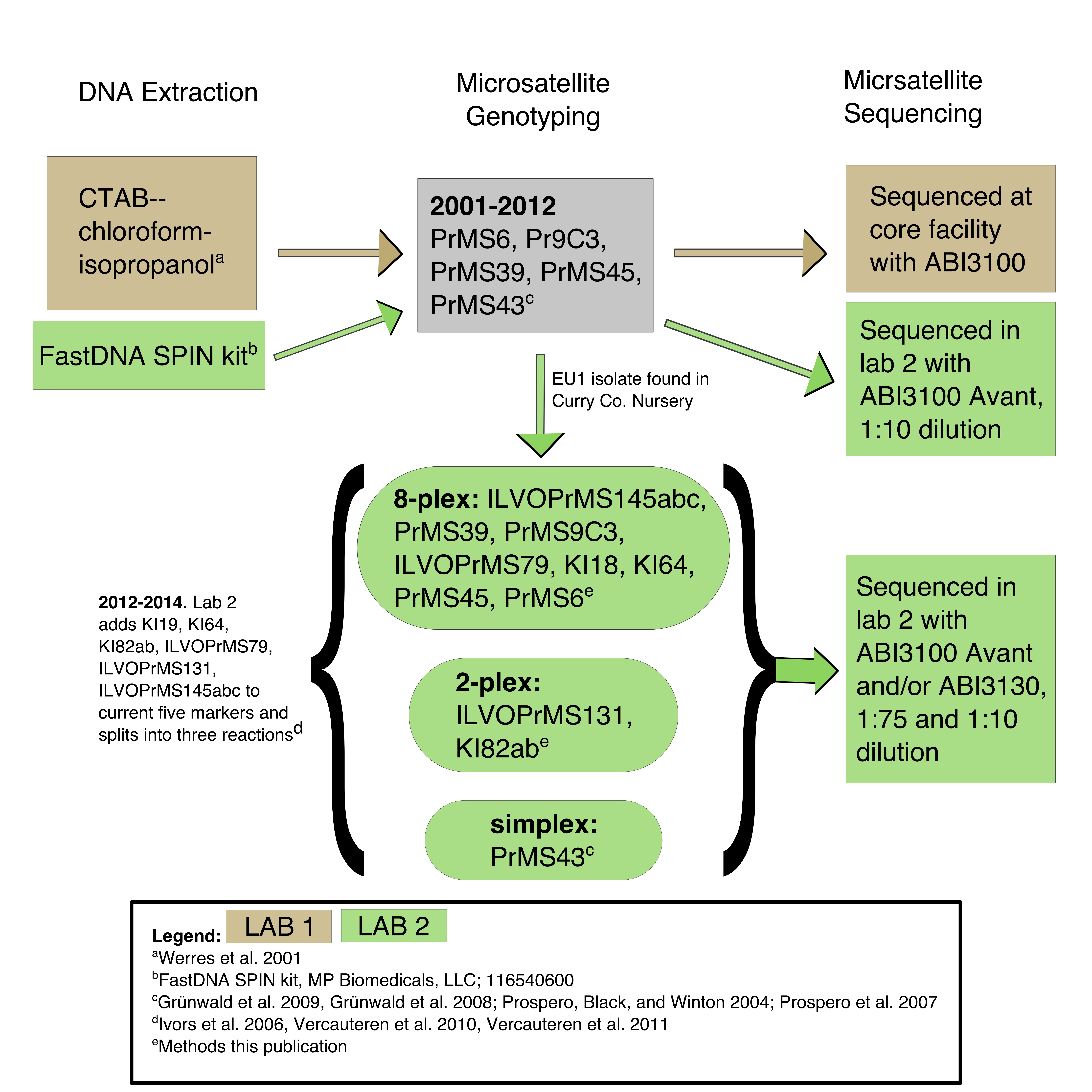
Figure 4.6: Diagram of DNA extraction, genotyping, and sequencing protocols utilized by two labs from 2001 to 2014. See supplementary text for details.

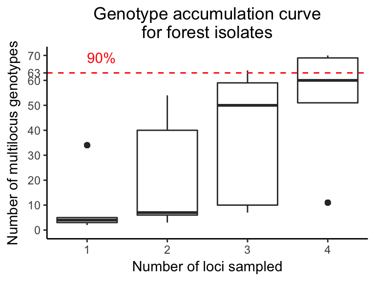
Figure 4.7: Genotype accumulation curve for OR forest P. ramorum isolates. The vertical axis denotes the number of observed MLGs, from 0 to the observed number of MLG in the forest populations, for a number of loci, indicated on the horizontal axis, randomly sampled without replacement. Each boxplot contains 1,000 random samples representing different possible combinations of n loci. The horizontal red dashed line represents 90% of MLG resolution.

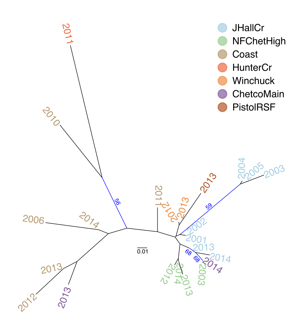
Figure 4.8: Neighbor joining tree based on Nei’s distance of the forest P. ramorum isolates by region with respect to year. Bootstrap values > 50% of 10,000 replicates are shown in blue.

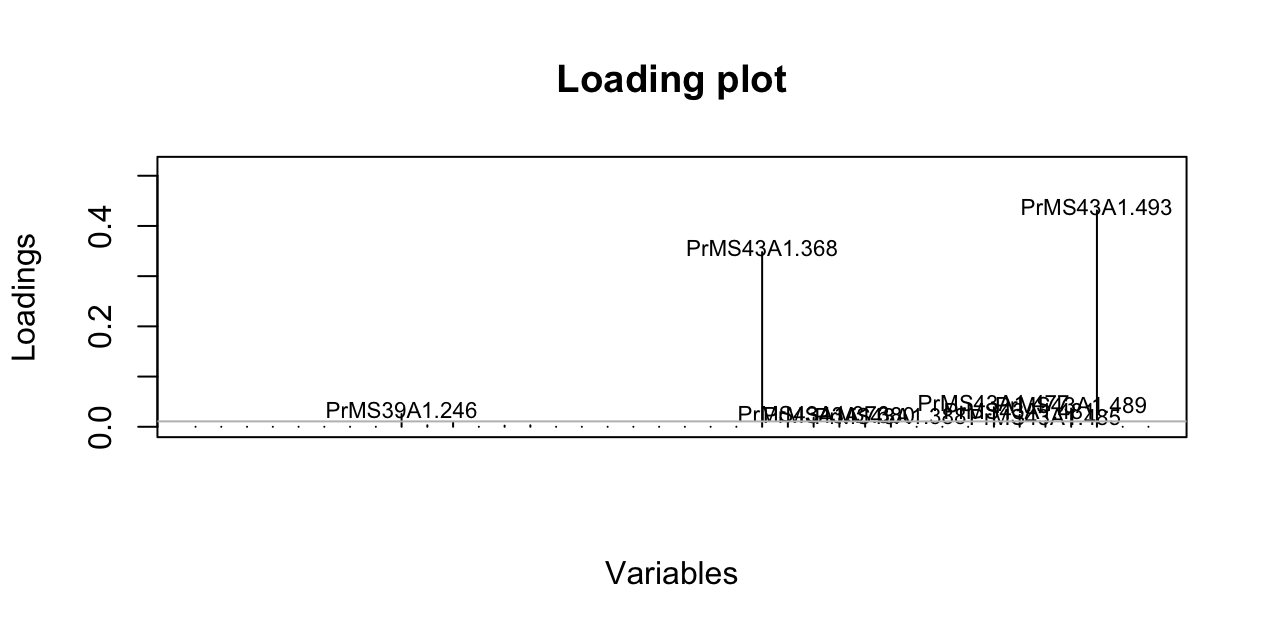
Figure 4.9: Loading plot from DAPC of P. ramorum from forest populations showing the contribution of alleles to the first DAPC eigenvalue separating Hunter Creek isolates from all other regions.

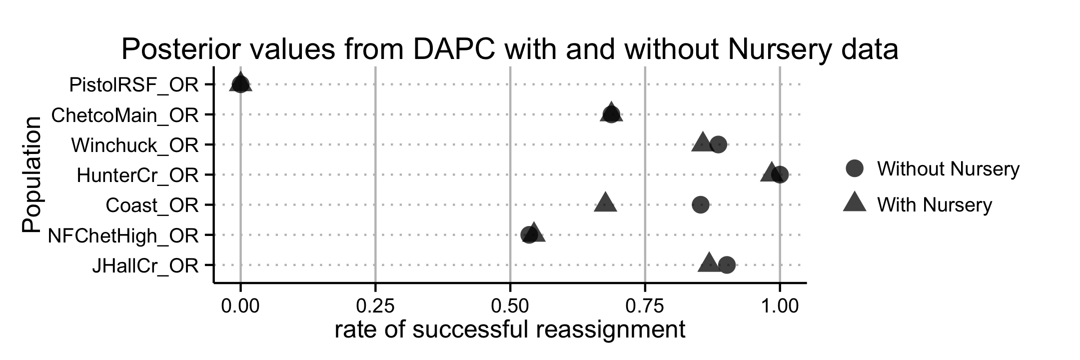
Figure 4.10: Fractions of posterior population assignments from DAPC clustering of P. ramorum isolates from forest populations. The horizontal axis represents the fraction of samples whose posterior group membership matched their prior group membership on the vertical axis. Shape indicates presence or absence of nursery populations in the DAPC.

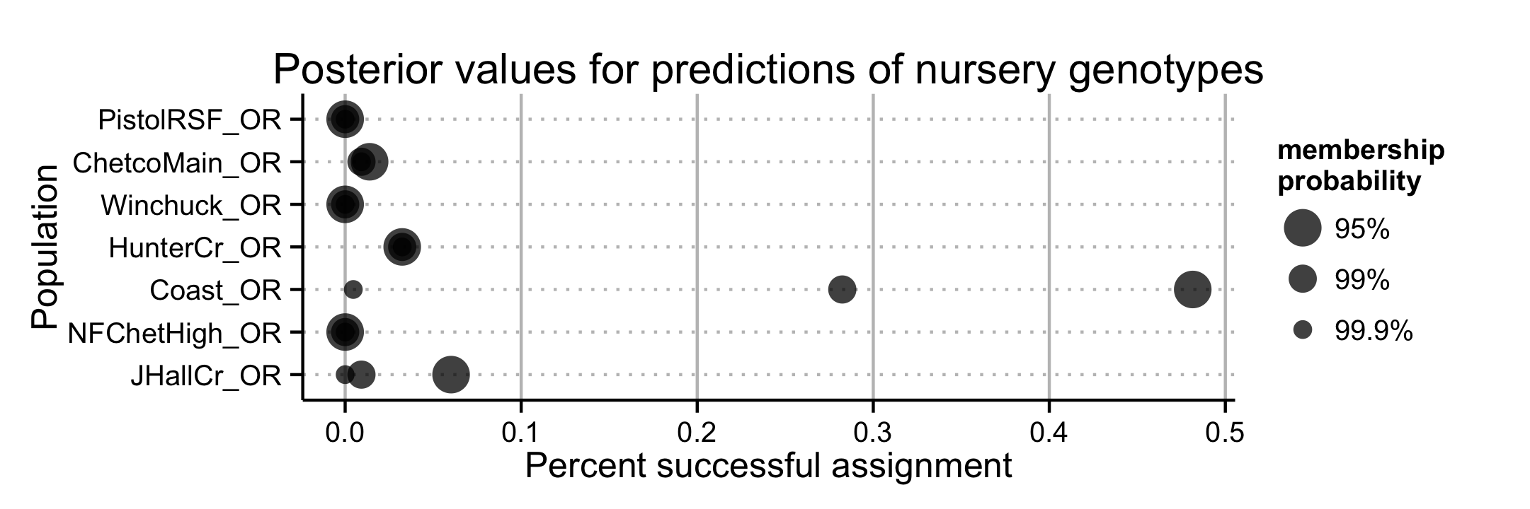
Figure 4.11: Prediction of nursery genotypes of P. ramorum into forest watershed regions. The horizontal axis indicates the fraction of nursery genotypes to be predicted to be similar to the populations on the vertical axis with a 95, 99, and 99.9% probability as indicated by the size of the points.

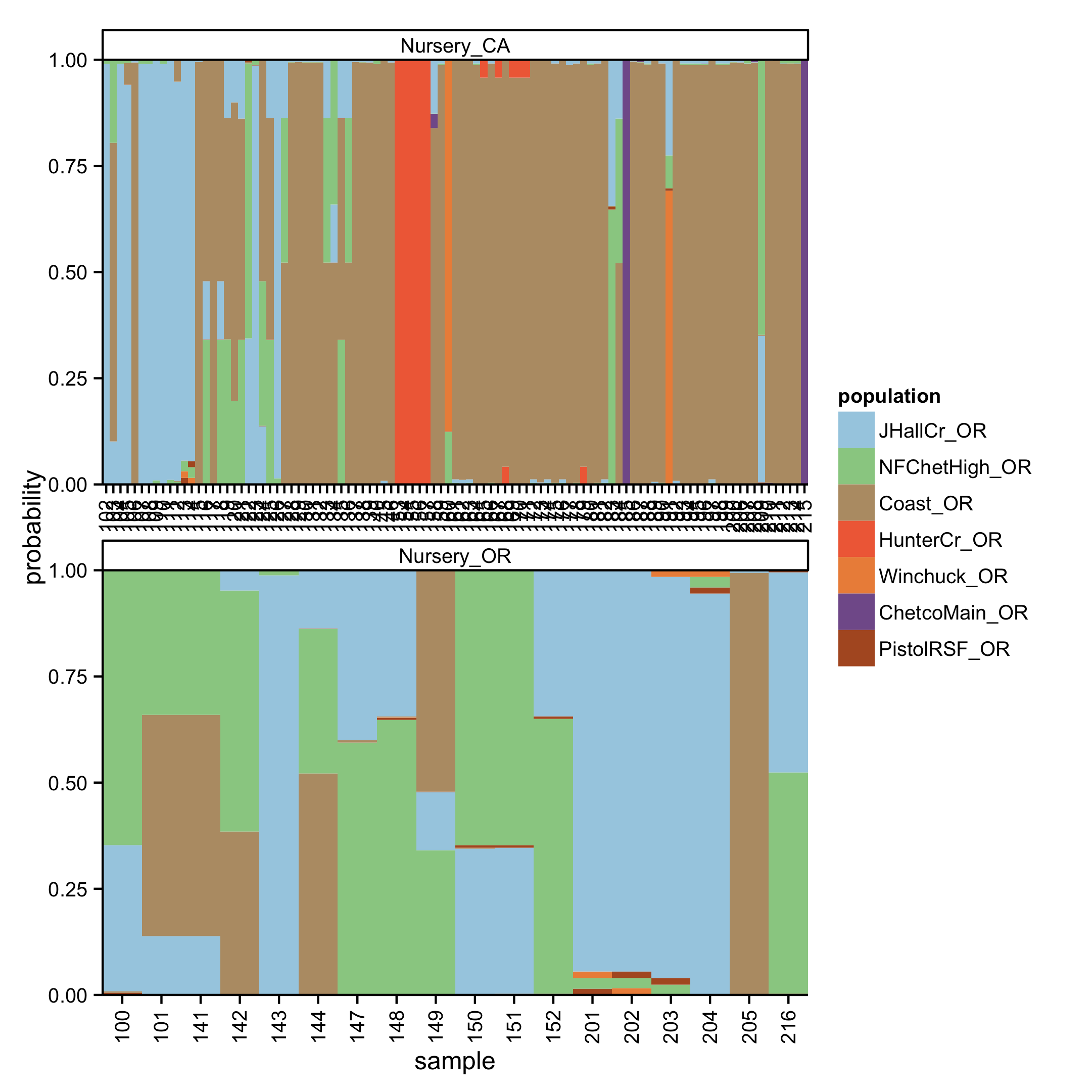
Figure 4.12: Graphical representation of prediction of nursery isolates of P. ramorum into forest watershed regions. Each column represents a different isolate. Colors within the columns represent membership probabilities from forest populations.

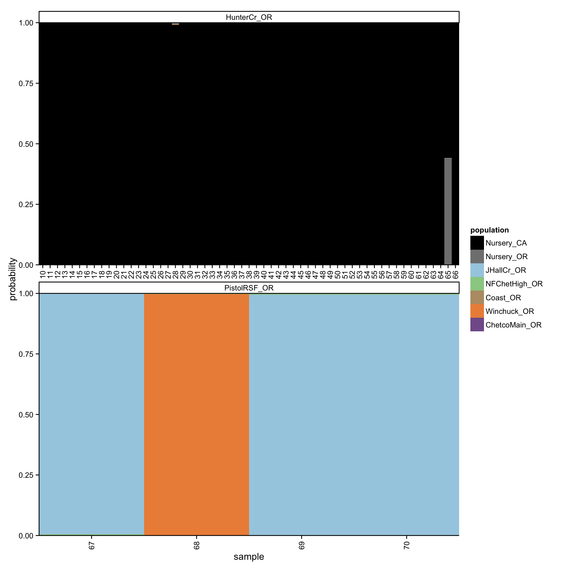
Figure 4.13: Graphical representation of predicted membership of P. ramorum isolates from Hunter Creek and Pistol River South Fork in forest and nursery populations. Each column represents a different isolate. Colors within the columns represent membership probabilities from the populations indicated in the legend.

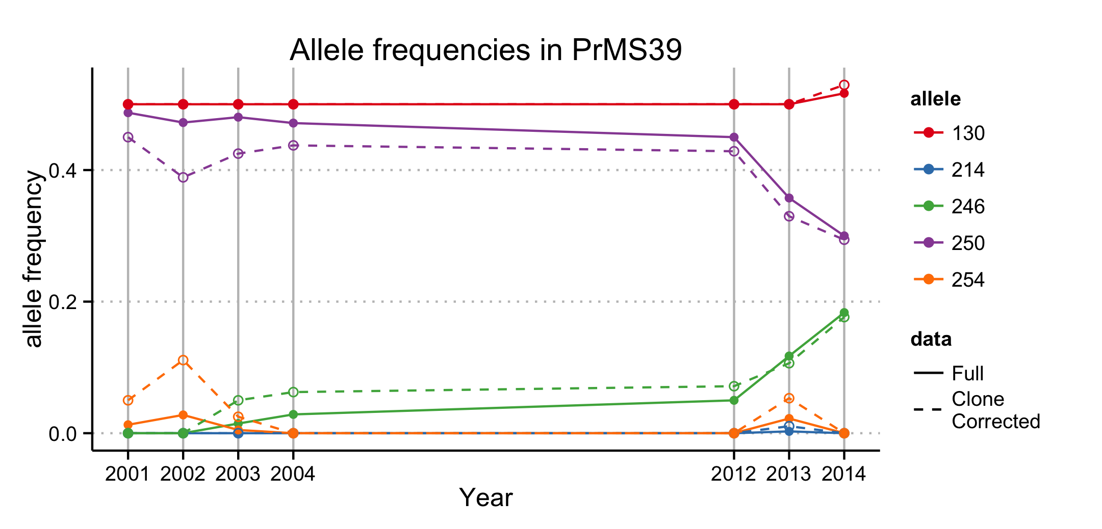
Figure 4.14: Allele frequencies of locus PrMS39 of P. ramorum across years of the forest populations. Years 2005 through 2011 have been omitted due to small sample sizes and outlier genotypes.

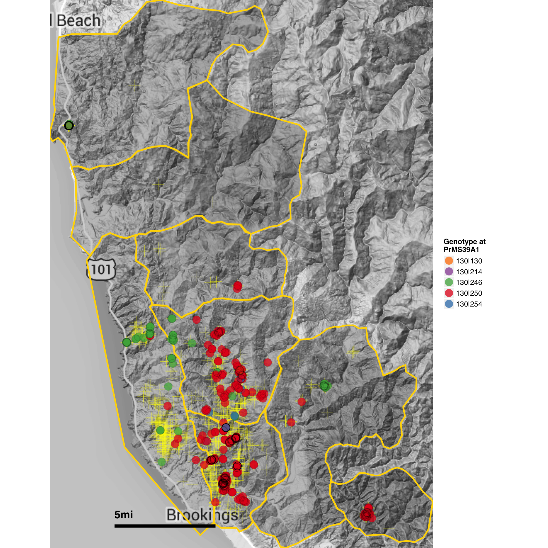
Figure 4.15: Map of the infected area in Curry county showing the P. ramorum genotypes at locus PrMS39. Each colored circle represents a different forest isolate while each yellow cross represents a sampled tree. Yellow borders denote different regions.

4.7.3 Supplementary Tables

Table 4.5: Mean allelic diversity metrics of clone-corrected populations of Phytophthora ramorum sampled in Curry County, Oregon between 2001-14 causing sudden oak death. MLG = Number of Multilocus Genotypes; alleles = Average number of alleles across 5 loci; 1-D = Simpson’s Index averaged across 5 loci; Hexp = Nei’s 1978 expected heterozygosity; Evenness = Evenness averaged across 5 loci

Population	MLG	alleles	1-D	Hexp	Evenness
ChetcoMain	7	3.0	0.58	0.97	0.94
Coast	12	3.8	0.59	0.97	0.96
HunterCr	4	2.6	0.56	0.96	0.95
JHallCr	30	4.4	0.57	0.91	0.89
NFChetHigh	35	4.8	0.60	0.90	0.89
PistolRSF	2	2.4	0.55	1.00	1.00
Winchuck	9	3.4	0.56	0.94	0.92
2001	10	3.6	0.56	0.94	0.91
2002	9	3.0	0.56	0.94	0.93
2003	20	4.2	0.56	0.90	0.89
2004	8	2.8	0.50	0.84	0.85
2005	2	2.4	0.50	0.90	0.92
2006	1	2.0	0.50	1.00	1.00
2010	1	2.0	0.50	1.00	1.00
2011	6	3.0	0.58	0.98	0.96
2012	7	3.2	0.58	0.96	0.95
2013	47	5.4	0.60	0.89	0.90
2014	17	3.8	0.59	0.97	0.93
pooled	70	6.0	0.60	0.89	0.90

Table 4.6: Allelic diversity metrics for each locus of clone-corrected Phytophthora ramorum data in Curry County, Oregon between 2001-14 causing sudden oak death. alleles = number of observed alleles; 1-D = Simpson’s Index; Hexp = Nei’s 1978 expected heterozygosity; E.5 = Evenness

locus	alleles	1-D	Hexp	E.5
PrMS6	2	0.50	0.99	0.99
Pr9C3	2	0.50	0.99	0.99
PrMS39	5	0.62	0.78	0.78
PrMS45	3	0.51	0.76	0.95
PrMS43	18	0.89	0.95	0.78
mean	6	0.60	0.89	0.90

Table 4.7: Genotypic diversity metrics or populations of Phytophthora ramorum sampled in Curry County, Oregon between 2001-14 causing sudden oak death. Pop = Population name (Total == Pooled) N = Census population size MLG = Number of unique multilocus genotypes (MLG) observed eMLG = Number of expected MLG based on rarefaction at smallest N >= 10 SE = Standard error of rarefaction analysis H = Shannon-Wiener Index of MLG diversity (95% CI in parentheses) G = Stoddart and Taylor’s Index of MLG diversity (95% CI in parentheses) E.5 = Evenness (95% CI in parentheses) rbarD = Standardized index of association p.rbarD = p-value for the standardized index of association based on 999 permutations NaN = Insufficient data for analysis

Population	N	MLG	eMLG	SE	H	G	E.5	rbarD	p.rD
2001	39	10	3.65	1.160	1.19 (0.61-1.48)	1.9 (1.38-2.81)	0.4 (0.4-0.57)	-0.068	0.999
2002	36	9	4.20	1.130	1.37 (0.79-1.64)	2.34 (1.52-3.52)	0.45 (0.43-0.65)	0.193	0.001
2003	102	20	4.75	1.300	1.81 (1.39-2)	2.92 (2.19-3.96)	0.38 (0.36-0.49)	0.143	0.001
2004	35	8	4.56	1.010	1.57 (1.12-1.76)	3.53 (2.3-4.77)	0.66 (0.56-0.84)	0.184	0.001
2005	2	2	2.00	0.000	0.69 (0-0.69)	2 (1-2)	1 (1-1)	NA	NA
2006	1	1	1.00	0.000	0 (0-0)	1 (1-1)	NaN (NA)	NA	NA
2010	1	1	1.00	0.000	0 (0-0)	1 (1-1)	NaN (NA)	NA	NA
2011	68	6	2.15	0.827	0.56 (0.26-0.79)	1.32 (1.13-1.59)	0.42 (0.38-0.56)	0.181	0.001
2012	20	7	5.01	0.916	1.62 (1.03-1.78)	4 (2.2-5.26)	0.74 (0.59-0.92)	-0.175	1.000
2013	179	47	7.74	1.200	3.15 (2.83-3.17)	13.8 (10.2-16.3)	0.57 (0.54-0.7)	0.029	0.001
2014	30	17	8.09	1.030	2.67 (2.08-2.61)	12.2 (6.16-12.2)	0.83 (0.69-0.93)	-0.006	0.555
JHallCr	244	30	4.89	1.330	1.97 (1.69-2.12)	3.13 (2.57-3.83)	0.34 (0.33-0.41)	0.103	0.001
NFChetHigh	114	35	6.81	1.340	2.74 (2.3-2.82)	7.07 (4.8-9.88)	0.42 (0.4-0.59)	0.066	0.001
Coast	34	12	5.91	1.170	2.05 (1.49-2.16)	5.56 (3.36-7.22)	0.68 (0.61-0.85)	0.283	0.001
HunterCr	66	4	1.88	0.690	0.42 (0.18-0.62)	1.24 (1.1-1.46)	0.46 (0.39-0.6)	-0.047	1.000
Winchuck	35	9	4.29	1.070	1.47 (0.95-1.7)	2.88 (1.89-4.15)	0.56 (0.49-0.77)	-0.014	0.756
ChetcoMain	16	7	5.00	0.926	1.45 (0.69-1.69)	2.84 (1.49-4.74)	0.56 (0.49-0.88)	0.396	0.001
PistolRSF	4	2	2.00	0.000	0.56 (0-0.69)	1.6 (1-2)	0.8 (0.8-1)	NA	NA
Total	513	70	6.95	1.330	2.98 (2.78-3.04)	8.64 (7.19-10.1)	0.41 (0.39-0.48)	0.082	0.001

References

Everhart, S. E., Tabima, J. F., & Grünwald, N. J. (2014). Phytophthora ramorum. In Genomics of plant-associated fungi and oomycetes: Dicot pathogens (pp. 159–174). Berlin, Heidelberg: Springer. https://doi.org/10.1007/978-3-662-44056-8_8

Grünwald, N. J., Goss, E. M., & Press, C. M. (2008a). Phytophthora ramorum: a pathogen with a remarkably wide host range causing Sudden Oak Death on oaks and ramorum blight on woody ornamentals. Molecular Plant Pathology, 9(6), 729–740. https://doi.org/10.1111/j.1364-3703.2008.00500.x

Hansen, E. M., Kanaskie, A., Prospero, S., McWilliams, M., Goheen, E. M., Osterbauer, N., Reeser, P., & Sutton, W. (2008). Epidemiology of Phytophthora ramorum in Oregon tanoak forests. Canadian Journal of Forest Research, 38(5), 1133–1143. https://doi.org/10.1139/x07-217

Rizzo, D. M., Garbelotto, M., & Hansen, E. M. (2005). Phytophthora ramorum: Integrative research and management of an emerging pathogen in California and Oregon forests. Annual Review of Phytopathology, 43(1), 309–335. https://doi.org/10.1146/annurev.phyto.42.040803.140418

Kamoun, S., Furzer, O., Jones, J. D. G., Judelson, H. S., Ali, G. S., Dalio, R. J. D., Roy, S. G., Schena, L., Zambounis, A., Panabières, F., Cahill, D., Ruocco, M., Figueiredo, A., Chen, X.-R., Hulvey, J., Stam, R., Lamour, K., Gijzen, M., Tyler, B. M., Grünwald, N. J., Mukhtar, M. S., Toé, D. F. A., Tör, M., Ackerveken, G. V. D., McDowell, J., Daayf, F., Fry, W. E., Lindqvist-Kreuze, H., Meijer, H. J. G., Petre, B., Ristaino, J., Yoshida, K., Birch, P. R. J., & Govers, F. (2014). The top 10 oomycete pathogens in molecular plant pathology. Molecular Plant Pathology, 16(4), 413–434. https://doi.org/10.1111/mpp.12190

Werres, S., Marwitz, R., Man In’t veld, W. A., de Cock, A. W., Bonants, P. J., de Weerdt, M., Themann, K., Ilieva, E., & Baayen, R. P. (2001). Phytophthora ramorum sp. nov., a new pathogen on Rhododendron and Viburnum. Mycological Research, 105(10), 1155–1165. https://doi.org/10.1016/s0953-7562(08)61986-3

Grünwald, N. J., Goss, E. M., Ivors, K., Garbelotto, M., Martin, F. N., Prospero, S., Hansen, E., Bonants, P. J. M., Hamelin, R. C., Chastagner, G., Werres, S., Rizzo, D. M., Abad, G., Beales, P., Bilodeau, G. J., Blomquist, C. L., Brasier, C., Bri‘ere, S. C., Chandelier, A., Davidson, J. M., Denman, S., Elliott, M., Frankel, S. J., Goheen, E. M., de Gruyter, H., Heungens, K., James, D., Kanaskie, A., McWilliams, M. G., in ‘t Veld, W. M., Moralejo, E., Osterbauer, N. K., Palm, M. E., Parke, J. L., Sierra, A. M. P., Shamoun, S. F., Shishkoff, N., Tooley, P. W., Vettraino, A. M., Webber, J., & Widmer, T. L. (2009). Standardizing the nomenclature for clonal lineages of the sudden oak death pathogen, Phytophthora ramorum. Phytopathology, 99(7), 792–795. https://doi.org/10.1094/phyto-99-7-0792

Ivors, K., Garbelotto, M., Vries, I. D. E., Ruyter-spira, C., Hekkert, B. T., Rosenzweig, N., & Bonants, P. (2006). Microsatellite markers identify three lineages of Phytophthora ramorum in US nurseries, yet single lineages in US forest and European nursery populations. Molecular Ecology, 15(6), 1493–1505. https://doi.org/10.1111/j.1365-294x.2006.02864.x

Prospero, S., Black, J. A., & Winton, L. M. (2004). Isolation and characterization of microsatellite markers in Phytophthora ramorum, the causal agent of Sudden Oak Death. Molecular Ecology Notes, 4(4), 672–674. https://doi.org/10.1111/j.1471-8286.2004.00778.x

Prospero, S., Grünwald, N. J., Winton, L. M., & Hansen, E. M. (2009). Migration Patterns of the Emerging Plant Pathogen Phytophthora ramorum on the West Coast of the United States of America. Phytopathology, 99(6), 739–749. https://doi.org/10.1094/phyto-99-6-0739

Prospero, S., Hansen, E. M., Grünwald, N. J., & Winton, L. M. (2007). Population dynamics of the Sudden Oak Death pathogen Phytophthora ramorum in Oregon from 2001 to 2004. Molecular Ecology, 16(14), 2958–2973. https://doi.org/10.1111/j.1365-294x.2007.03343.x

Grünwald, N. J., Garbelotto, M., Goss, E. M., Heungens, K., & Prospero, S. (2012). Emergence of the Sudden Oak Death pathogen Phytophthora ramorum. Trends in Microbiology, 20(3), 131–138. https://doi.org/10.1016/j.tim.2011.12.006

Poucke, K. V., Franceschini, S., Webber, J. F., Vercauteren, A., Turner, J. A., McCracken, A. R., Heungens, K., & Brasier, C. M. (2012). Discovery of a fourth evolutionary lineage of Phytophthora ramorum: EU2. Fungal Biology, 116(11), 1178–1191. https://doi.org/10.1016/j.funbio.2012.09.003

Mascheretti, S., Croucher, P. J. P., Vettraino, A., Prospero, S., & Garbelotto, M. (2008). Reconstruction of the Sudden Oak Death epidemic in California through microsatellite analysis of the pathogen Phytophthora ramorum. Molecular Ecology, 17(11), 2755–2768. https://doi.org/10.1111/j.1365-294x.2008.03773.x

Goss, E. M., Larsen, M., Chastagner, G. A., Givens, D. R., & Grünwald, N. J. (2009). Population genetic analysis infers migration pathways of Phytophthora ramorum in US nurseries. PLoS Pathogens, 5(9), e1000583. https://doi.org/10.1371/journal.ppat.1000583

Goss, E. M., Larsen, M., Vercauteren, A., Werres, S., Heungens, K., & Grünwald, N. J. (2011). Phytophthora ramorum in Canada: Evidence for migration within North America and from Europe. Phytopathology, 101(1), 166–171. https://doi.org/10.1094/phyto-05-10-0133

Winton, L. M., & Hansen, E. M. (2001). Molecular diagnosis of Phytophthora lateralis in trees, water, and foliage baits using multiplex polymerase chain reaction. Forest Pathology, 31(5), 275–283. https://doi.org/10.1046/j.1439-0329.2001.00251.x

Grünwald, N. J., Kitner, M., McDonald, V., & Goss, E. M. (2008b). Susceptibility in Viburnum to Phytophthora ramorum. Plant Disease, 92(2), 210–214. https://doi.org/10.1094/pdis-92-2-0210

Vercauteren, A., Dobbelaere, I. D., Grünwald, N. J., Bonants, P., van Bockstaele, E., Maes, M., & Heungens, K. (2010). Clonal expansion of the Belgian Phytophthora ramorum populations based on new microsatellite markers. Molecular Ecology, 19(1), 92–107. https://doi.org/10.1111/j.1365-294x.2009.04443.x

Vercauteren, A., Larsen, M., Goss, E., Grünwald, N. J., Maes, M., & Heungens, K. (2011). Identification of new polymorphic microsatellite markers in the NA1 and NA2 lineages of Phytophthora ramorum. Mycologia, 103(6), 1245–1249. https://doi.org/10.3852/10-420

R Core Team. (2014). R: A language and environment for statistical computing. Vienna, Austria: R Foundation for Statistical Computing. Retrieved from https://www.R-project.org/

Csardi, G., & Nepusz, T. (2006). The igraph software package for complex network research. InterJournal, Complex Systems, 1695. Retrieved from http://igraph.org

Kahle, D., & Wickham, H. (2013). ggmap: Spatial Visualization with ggplot2. The R Journal, 5(1), 144–161. Retrieved from http://journal.r-project.org/archive/2013-1/kahle-wickham.pdf

Kamvar, Z. N., Tabima, J. F., & Grünwald, N. J. (2014b). Poppr : an R package for genetic analysis of populations with clonal, partially clonal, and/or sexual reproduction. PeerJ, 2, e281. https://doi.org/10.7717/peerj.281

Paradis, E., Claude, J., & Strimmer, K. (2004). APE: Analyses of phylogenetics and evolution in R language. Bioinformatics, 20(2), 289–290. https://doi.org/10.1093/bioinformatics/btg412

Wickham, H. (2009). ggplot2: Elegant Graphics for Data Analysis. Springer-Verlag New York. Retrieved from http://ggplot2.org

Bivand, R., Keitt, T., & Rowlingson, B. (2014). rgdal: Bindings for the Geospatial Data Abstraction Library. Retrieved from https://CRAN.R-project.org/package=rgdal

Shannon, C. E. (1948). A mathematical theory of communication. ACM SIGMOBILE Mobile Computing and Communications Review, 5(1), 3–55.

Stoddart, J. A., & Taylor, J. F. (1988). Genotypic diversity: Estimation and prediction in samples. Genetics, 118(4), 705–11.

Grünwald, N. J., Goodwin, S. B., Milgroom, M. G., & Fry, W. E. (2003). Analysis of genotypic diversity data for populations of microorganisms. Phytopathology, 93(6), 738–746. https://doi.org/10.1094/phyto.2003.93.6.738

Ludwig, J. A., & Reynolds, J. F. (1988). Statistical ecology: A primer in methods and computing (Vol. 1). John Wiley & Sons.

Pielou, E. (1975). Ecological diversity. New York: Wiley & Sons.

Oksanen, J., Blanchet, F. G., Kindt, R., Legendre, P., Minchin, P. R., O’Hara, R. B., Simpson, G. L., Solymos, P., Stevens, M. H. H., & Wagner, H. (2013). Vegan: Community ecology package. Retrieved from https://CRAN.R-project.org/package=vegan

Canty, A., & Ripley, B. D. (2015). Boot: Bootstrap r (s-plus) functions. Retrieved from https://CRAN.R-project.org/package=boot

Heck, K. L., van Belle, G., & Simberloff, D. (1975). Explicit calculation of the rarefaction diversity measurement and the determination of sufficient sample size. Ecology, 56(6), 1459–1461. https://doi.org/10.2307/1934716

Hurlbert, S. H. (1971). The nonconcept of species diversity: A critique and alternative parameters. Ecology, 52(4), 577–586. https://doi.org/10.2307/1934145

Bruvo, R., Michiels, N. K., D’Souza, T. G., & Schulenburg, H. (2004). A simple method for the calculation of microsatellite genotype distances irrespective of ploidy level. Molecular Ecology, 13(7), 2101–2106.

Dray, S., & Dufour, A.-B. (2007). The ade4 package: Implementing the duality diagram for ecologists. Journal of Statistical Software, 22(4). https://doi.org/10.18637/jss.v022.i04

Mantel, N. (1967). The detection of disease clustering and a generalized regression approach. Cancer Research, 27(2 Part 1), 209–220.

Excoffier, L., Smouse, P. E., & Quattro, J. M. (1992). Analysis of molecular variance inferred from metric distances among DNA haplotypes: Application to human mitochondrial DNA restriction data. Genetics, 131(2), 479–91.

Jombart, T., Devillard, S., & Balloux, F. (2010). Discriminant analysis of principal components: A new method for the analysis of genetically structured populations. BMC Genetics, 11(1), 94. https://doi.org/10.1186/1471-2156-11-94

Rizzo, D. M., Garbelotto, M., Davidson, J. M., Slaughter, G. W., & Koike, S. T. (2002). Phytophthora ramorum as the cause of extensive mortality of Quercus spp. and Lithocarpus densiflorus in California. Plant Disease, 86(3), 205–214. https://doi.org/10.1094/pdis.2002.86.3.205

Mascheretti, S., Croucher, P. J. P., Kozanitas, M., Baker, L., & Garbelotto, M. (2009). Genetic epidemiology of the Sudden Oak Death pathogen Phytophthora ramorum in California. Molecular Ecology, 18(22), 4577–4590. https://doi.org/10.1111/j.1365-294x.2009.04379.x

Eyre, C. A., Kozanitas, M., & Garbelotto, M. (2013). Population dynamics of aerial and terrestrial populations of Phytophthora ramorum in a California forest under different climatic conditions. Phytopathology, 103(11), 1141–1152. https://doi.org/10.1094/phyto-11-12-0290-r

Croucher, P. J. P., Mascheretti, S., & Garbelotto, M. (2013). Combining field epidemiological information and genetic data to comprehensively reconstruct the invasion history and the microevolution of the Sudden Oak Death agent Phytophthora ramorum (Stramenopila: Oomycetes) in California. Biological Invasions, 15(10), 2281–2297. https://doi.org/10.1007/s10530-013-0453-8

Grünwald, N. J., & Goss, E. M. (2011). Evolution and population genetics of exotic and re-emerging pathogens: Novel tools and approaches. Annual Review of Phytopathology, 49(1), 249–267. https://doi.org/10.1146/annurev-phyto-072910-095246

Elshire, R. J., Glaubitz, J. C., Sun, Q., Poland, J. A., Kawamoto, K., Buckler, E. S., & Mitchell, S. E. (2011). A robust, simple genotyping-by-sequencing (GBS) approach for high diversity species. PLoS ONE, 6(5), e19379. https://doi.org/10.1371/journal.pone.0019379

Brownstein, M. J., Carpten, J. D., & Smith, J. R. (1996). Modulation of non-templated nucleotide addition by Taq DNA polymerase: Primer modifications that facilitate genotyping. BioTechniques, 20(6), 1004–6, 1008–10.