Chapter 5 Factors Influencing Inference of Clonality in Diploid Populations

Zhian N. Kamvar and Niklaus J. Grünwald

Target Journal: Molecular Ecology

5.1 Abstract

The index of association is a measure of multilocus linkage disequilibrium, which reflects the deviation of observed genetic variation from expected. In sexual populations, loci are randomly assorting due to recombination, resulting in a near-zero value of the index of association. In clonal populations, recombination is non-existent, meaning that loci are passed from parent to offspring in a non-independent fashion, resulting in a significantly non-zero value of the index of association. We build on previous work by investigating the effect of sample size, mutation rate, and clone correction on the power of the index of association to detect clonal reproduction in simulated data sets generated with microsatellite and genomic markers. Our findings suggest that power decreases with small sample sizes and low allelic diversity, and physical linkage in genomic markers does not affect power if permutation tests are performed with linkage groups. We hope that these novel insights provide useful to the study of molecular pathogens.

5.2 Introduction

Population genetic theory is largely based on model populations such as the neutral Wright-Fisher model in which populations are assumed to be infinitely large, with discrete generations, randomly assorting alleles, with no migration and no mutation (Hartl & Clark, 2007; Nielsen & Slatkin, 2013). By using such reductionist models, population geneticists are able to reduce the complexity and enable analyses to ask fundamental questions and test hypotheses about evolutionary processes that could explain population structure and history.

These neutral models, however, cannot be applied to populations whose life history violate the fundamental assumption of random assortment of alleles, such as populations that undergo clonal reproduction (Milgroom, 1996; Orive, 1993). For many clonal populations, the contribution of genetic variation from mutation is greater than that of recombination. While this increases the risk of the accumulation of deleterious mutations, the two-fold cost of sex is drastically reduced, meaning that selectively advantageous combinations of alleles are maintained (Heitman et al., 2012).

Pathogenic microorganisms can reproduce sexually or clonally (Milgroom, 1996; Tibayrenc, 1996). Diseases caused by these organisms are in part managed by the use of antimicrobial compounds that kill these organisms. Detecting recombination in populations of pathogenic microorganisms is therefore important for the implementation of rational management strategies as a prevalence of sexual reproduction could lead to the repeated emergence of novel, resistant genotypes (de Meeûs et al., 2006; Goss et al., 2014; Milgroom, 1996; Nieuwenhuis & James, 2016; Smith et al., 1993).

Several studies have attempted to infer the degree of sex in populations that undergo clonal reproduction (Ali et al., 2016; Balloux et al., 2003; de Meeûs & Balloux, 2004; Nieuwenhuis & James, 2016; Smith et al., 1993). For populations with well-defined sexual and clonal phases occurring at separate times, such as rust fungi, methods like CloNcaSe are effective for estimating the rate of sexual reproduction and effective population size (Ali et al., 2016). However, this method cannot be applied to populations where the reproductive cycle is not partitioned into discrete generations.

Simply detecting the presence of clonal reproduction, however can be useful in and of itself (Milgroom, 1996). A method commonly used to assess this is the index of association ($I_A$), and its standardized version, $\bar{r}_d$, which measure multilocus linkage disequilibrium (Agapow & Burt, 2001; Brown et al., 1980; de Meeûs & Balloux, 2004; Haubold et al., 1998; Kamvar et al., 2014 b; Smith et al., 1993). The value of $I_A$, as shown in equation (5.1), is measured as the ratio of observed variance ($V_O$) and expected variance ($V_E$) in genetic distance between samples (Agapow & Burt, 2001; Smith et al., 1993):

\[\begin{equation} I_A = \frac{V_O}{V_E} - 1 \tag{5.1} \end{equation}\]

The expected variance is practically modeled as the sum of the variances over m loci: $V_E = \sum^m{var_j}$ (Agapow & Burt, 2001; Haubold et al., 1998). If the differences between samples are randomly distributed (linkage equilibrium), we can expect the value of $I_A$ to be zero (Agapow & Burt, 2001; Smith et al., 1993). Under scenarios of non-random mating (e.g. population structure or clonal reproduction), the observed variance would be greater than the expected variance due to a multi-modal distribution of distances, and $I_A$ would be greater than zero (Agapow & Burt, 2001; Milgroom, 2015; Smith et al., 1993). Agapow & Burt (2001) noted that this metric does not have an upper limit and increases with the number of loci. To correct this, they developed $\bar{r}_d$ (equation (5.2)), which has a similar structure to a correlation coefficient and ranges from 0 (no linkage) to 1 (complete linkage):

\[\begin{align} % This mode aligns the equations to the '&=' signs \begin{split} % This mode groups the equations into one. \bar{r}_d &= \frac{\sum\sum{cov_{j,k}}}{ \sum\sum{\sqrt{var_{j} \cdot var_{k}}}} \\ &= \frac{V_O - V_E}{2\sum\sum{\sqrt{var_{j} \cdot var_{k}}}} \end{split} \tag{5.2} \end{align}\]

De Meeûx & Balloux (2004) investigated the effect of increasing levels of sexual reproduction on $\bar{r}_d$ (noted in their publication as $\bar{r}_D$). They found that very little ($\sim$ 1%) sexual reproduction is required to produce a value of $\bar{r}_d$ close to zero. This indicates that $\bar{r}_d$ alone might not be well suited as a measure of clonal reproduction. Prugnolle & de Meeûs (2010) tested the effect of sampling design on $\bar{r}_d$, finding that its value is drastically reduced when clones from multiple populations are sampled, leading to an over-estimation of the level of recombination.

These studies laid the groundwork for understanding the behavior of $\bar{r}_d$ under different scenarios of non-random mating in diploid organisms, but there were some limitations in available technology. For both studies, the only software available for calculation of $\bar{r}_d$ for diploid organisms was Multilocus, which could only take one data set at a time (Agapow & Burt, 2001; de Meeûs & Balloux, 2004; Kamvar et al., 2014 b; Prugnolle & de Meeûs, 2010). This constrained researchers to only analyze a minimal set of 20 populations per scenario.

A non-zero value of $I_A$ and $\bar{r}_d$ does not always indicate a significant departure from the null assumption of unlinked loci. Since the distribution of $I_A$ and $\bar{r}_d$ are not known, the safest way to test for significance are random permutation tests. These tests effectively create unlinked populations by shuffling individuals at each locus, independently and re-calculating $I_A$ and $\bar{r}_d$ (Agapow & Burt, 2001; Haubold et al., 1998; Smith et al., 1993). An upper one-sided test of significance is then used to see if the observed statistic is greater than the observed distribution.

Standard practice for analyzing microbial populations is to perform this test on both the whole data set (wd) and clone-corrected data (cc), where each multilocus genotype is represented only once per population to avoid signatures of linkage that arise from re-sampling the same individual (Goss et al., 2014; McDonald, 1997; Milgroom, 1996). If the p-value for $\bar{r}_d$ is significant after clone-correction, then the population is expected to be clonal. While significance testing is available in Multilocus in the form of random permutations, it is computationally expensive, and can only take one data set at a time (Agapow & Burt, 2001; Kamvar et al., 2014 b). As a result, power analysis of $\bar{r}_d$ to detect clonal reproduction with and without clone-correction has not yet been performed (de Meeûs & Balloux, 2004).

In the years since the studies conducted by de Meeûs & Balloux (2004) and Prugnolle & de Meeûs (2010), reduced-representation, high-throughput sequencing methods such as Genotyping-By-Sequencing (GBS) and Restriction site associated DNA sequencing (RAD-seq) have become popular tools for population genetic analysis (Davey & Blaxter, 2010; Davey et al., 2011; Elshire et al., 2011). These methods have the capability to generate thousands of unlinked markers at a fraction of the cost and time necessary to develop high quality microsatellite markers. These marker systems are also prone to missing data and high error rates (Mastretta-Yanes et al., 2014). The index of association was developed for multiple loci at a time when obtaining even 100 unlinked markers posed a significant challenge. With the advent of these technologies, it is unclear how marker choice and genotyping error affect the index of association.

We developed the R package poppr for analysis of clonal populations, removing the limitations of data input and computational expense of analyzing the index of association (Kamvar et al., 2014 b) and further expanded this to analysis of genome-wide SNP data (Kamvar et al., 2015 a; R Core Team, 2016). With these tools we expand on previous studies by asking how sample size, marker choice, clone-correction, and the assumption of homogeneous mutation rates affect our ability to detect clonal reproduction in diploid populations. Our objectives to answer these questions are to (1) re-analyze $\bar{r}_d$ against increasing rates of sexual reproduction in both microsatellite and SNP data sets, (2) perform a power analysis of $\bar{r}_d$ to assess sensitivity and specificity, and (3) assess how genotypic and allelic evenness and diversity affects $\bar{r}_d$. Because studies have observed significantly negative values of $I_A$ and $\bar{r}_d$ (p $\geq$ 0.95), we additionally seek to determine what factors result in negative $\bar{r}_d$ values. This work provides novel insights into the sensitivity and scope of the index of association for inferring clonality.

5.3 Methods

We used simulations to evaluate the behavior of $\bar{r}_d$ under different population scenarios. Initial sets of simulations were created for different levels of sexual reproduction for each marker type. All simulations were performed with the python package simuPOP version 1.1.7 in python version 3.4 (Peng & Amos, 2008). For each scenario, 100 simulations with 10 replicates were created with a census size of 10,000 diploid individuals with equal mating type proportions evolved over 10,000 generations. We chose a census size of 10,000 individuals to minimize the effect of drift. We chose to run the simulations for 10,000 generations because this was previously shown in de Meeûs & Balloux (2004) to be sufficient in reaching equilibrium for summary statistics.

The simulated populations were first stored in the native simuPOP format and then transferred to feather format using the python and R packages feather version 0.3.0 for downstream analyses. Microsatellite simulations were performed on Ubuntu Linux version 14.04; SNP simulations were performed on CentOS Linux version 6.8. During downstream analysis, 10, 25, 50, and 100 individuals were sampled without replacement for each replicate in R version 3.2 with the package poppr version 2.3.0 (Kamvar et al., 2015 a, 2014 b; R Core Team, 2016). Analyses (described below) were performed on both full and clone-corrected data sets. All downstream analyses were run on the OSU CGRB Core Computing Facility.

5.3.1 Simulating Microsatellite Loci

Each population was simulated with 21 co-dominant, unlinked loci containing 6 to 10 alleles per locus with frequencies drawn from a uniform distribution and subsequently normalized so that allele frequencies at each locus sum to one. We used 6 to 10 alleles per locus as this is the number of alleles commonly used for population genetic studies to avoid statistical noise. Before mating, mutations occurred at each locus at a rate of 1e-5 mutations/generation with the exception of the first locus, at which the mutation rate was set to 1e-3. The mutation rate of 1e-5 was selected as this was previously used in de Meeûs & Balloux (2004) and is close to the estimated recombination rate of Saccharomyces cerevisiae microsatellite loci (Lynch et al., 2008). All mutations were applied in a stepwise manner using the StepwiseMutator() operator in simuPOP.

5.3.2 Simulating SNP Loci

Simulations of 10,000 diploid, biallelic loci spread evenly over 10 chromosomal fragments were simulated with a mutation rate of 1e-5 mutations per generation for forward and backward mutations using the SNPMutator() operator and and a recombination rate of 0.01 between adjacent loci using the Recombinator() operator in simuPOP.

5.3.3 Mating

Simulations of sexual reproduction were conducted at 10 rates of sexual reproduction over a log scale (0.0, 1e-4, 5e-4, 1e-3, 5e-3, 1e-2, 5e-2, 0.1, 0.5, 1.0) reflecting the fraction of individuals in generation t+1 produced via sexual reproduction. One to three offspring could be produced at each mating event. Rates were chosen to investigate the dynamics of $\bar{r}_d$ at low levels of clonal reproduction. For sexual events, two parents were chosen randomly from the population with the RandomSelection() operator and offspring genotypes were created via the MendelianGenoTransmitter() operator. The clonal fraction was created by randomly sampling individuals from the population and duplicating their genotypes with the CloneGenoTransmitter() operator. If one mating type was lost before 10,000 generations, the simulation would continue to completion with only clonal reproduction.

5.3.4 Analysis of Microsatellite Data

The standardized index of association ($\bar{r}_d$, Agapow & Burt (2001)) was calculated for full and clone-corrected data using the poppr function ia() (Kamvar et al., 2014 b). Tests for significance were performed by randomly permuting the alleles at each locus independently and then assessing $\bar{r}_d$. A total of 999 permutations were conducted for each replicate population to evaluate statistical support. Analyses were done for both full and clone-corrected data. The p-values reflect the proportion of observations greater than the observed statistic. Estimates of genotypic diversity were assessed with the poppr function diversity_boot() with 999 bootstrap replicates, recording the estimate and variance (Kamvar et al., 2015 a). The genotypic diversity statistics we calculated were Shannon’s Index, $H = -\sum p_i ln p_i$ (Shannon, 1948), Stoddart and Taylor’s Index, $G = 1/\sum p_i^2$ (Stoddart & Taylor, 1988), and Evenness, $E_5 = (G - 1)/(e^H - 1)$ (Pielou, 1975) where $p_i$ is the frequency of the ith genotype. We additionally calculated Nei’s expected heterozygosity, also known as gene diversity (Nei, 1978), and mean allelic evenness $E_{5A} = (1/m) \sum E_{5l}$, where m is the number of loci and $E_{5l}$ is the evenness of the alleles at locus l with the poppr function locus_table() (Grünwald et al., 2003; Kamvar et al., 2014 b).

5.3.5 Analysis of SNP Data

The overall value of $\bar{r}_d$ was calculated for each simulation with the poppr function bitwise.ia() (Kamvar et al., 2015 a). Significance was first assessed by randomly shuffling genotypes at each locus independently and then, to preserve existing background linkage structure, at each chromosome independently. This was done 999 times for each replicate population. P-values represent the proportion of random samples greater than or equal to the observed statistic.

Because GBS data are associated with high error rates, we additionally wanted to assess the effect of missing data on analysis. To do this, we used scripts written for Kamvar et al. (2015 a) to randomly insert missing data via the pop_NA() function (Kamvar et al., 2015 b) at rates of 1%, 5%, and 10% each.

5.3.6 Power Analysis

Permutation analysis of the index of association is commonly used to calculate statistical support for detecting non-random mating. If the observed value of $\bar{r}_d$ is greater than 95% of the results from the permutations, then the null hypothesis of linkage equilibrium is rejected. The power or sensitivity of this test can be seen as the fraction of significant results within a set of simulation parameters when the rate of sexual reproduction is < 1.

The Receiver Operating Characteristic (ROC) curve is a statistical method of assessing the balance between sensitivity and specificity of a diagnostic method (Metz, 1978). This is done by simultaneously assessing the true positive fraction of tests to a false positive fraction along a gradient of thresholds of increasing leniency. A simple way of thinking about ROC analysis is to imagine two factories that both make marbles. On average, factory A makes marbles half the size of factory B. Both factories manufacture for the same distributor, which mixes the marbles from both factories. You are tasked with finding the best sieve that can accurately and precisely separate the marbles. To measure this quantity, you order a set of orange marbles from factory A and a set of blue marbles from factory B. To calculate the ROC curve, you would take a range of sieves and stack them such that the one with the largest mesh size is on top and the one with the smallest mesh size is on the bottom and pour both orange and blue marbles through. The fractions of orange and blue marbles that passed through each sieve are the true positive and false positive fractions, respectively. Plot the true positive fraction against the false positive fraction for each sieve respectively, and you can assess how well the sieve method works by examining the shape of the ROC curve.

A useful summary of the ROC curve is to calculate the area under the ROC curve (AURC). Briefly, if a method has perfect explanatory power, the area under the ROC curve will be equal to 1. If a method has no explanatory power, the AURC will be equal to 0.5. We used this method to assess the efficacy of $\bar{r}_d$ to detect non-random mating.

To calculate the ROC curve, we first define what a positive value is. If we consider the p-value of $\bar{r}_d$ as a classifier to determine clonality, we can define the false positive fraction as the fraction of observations where $p \leq \alpha$ for simulations where the rate of sexual reproduction is set to 1.0 (Table 5.1). In contrast, the true positive fraction is the fraction of observations where $p \leq \alpha$ in simulations where clonality is introduced (e.g. all simulations where the rate of sexual reproduction is less than 1.0).

Table 5.1: Definitions of false positive and true positive values for ROC analysis of simulations. p is the p-value for $\bar{r}_d$, $\alpha$ is a threshold value in [0, 1]. Randomly mating populations are simulated with a sex rate of 1. Non-Random mating populations are simulated with a sex rate less than one.
Reproductive Mode	$p \leq \alpha$	$p > \alpha$
Non-Random Mating	True Positive	False Negative
Random Mating	False Positive	True Negative

We constructed each ROC curve by plotting the true positive fraction on the y axis and the false positive fraction on the x axis with values of $\alpha$ in increments of 0.01 from 0 to 1. Curves were calculated hierarchically by rate of sexual reproduction (< 1) and a unique seed was used to generate the populations. For each hierarchical level, separate curves were calculated for sample size, mutation rate, and clone-correction. The areas under the ROC curves (AURC) were calculated using the auc() function in the R package flux version 0.3-0 (Jurasinski et al., 2014).

Because simulations across rates of sexual reproduction were generated from unique seeds, we additionally constructed ROC curves for each seed with respect to clone-correction, sample size, and mutation rate. To test for significant effects of clone-correction, sample size, and mutation rate on the inference of non-random mating on microsatellite data, we then separated the data by rate of sexual reproduction and performed a three way (type III) ANOVA on each rate separately with formula (5.3). For SNP data, we did not have clone correction or mutation rate differences, so we set these variables to 1.

\[\begin{equation} AURC \sim Clone Correction \times Sample Size \times Mutation Rate \tag{5.3} \end{equation}\]

Because of a pattern that we saw in the results of $E_{5A}$ for microsatellite data, we asked whether or not using a value of $E_{5A} \geq 0.85$ could help detect clonal reproduction even if the p-value was non-significant. To assess this, we conducted an additional ROC analysis to condition p-values on $E_{5A}$ such that non-significant values that also had $E_{5A} \geq 0.85$ would be considered significant.

5.4 Results

5.4.1 Clone Correction Negatively Impacts Clonal Inference

For microsatellite data, the values of $\bar{r}_d$ for completely clonal and nearly clonal populations ranged from -0.577 to 1 in completely clonal data sets (Fig. 5.1). Genotypic diversity statistics (Fig. 5.2, top six panels) showed a predictable pattern of genotypic diversity increasing with sexual reproduction with diversity being higher on average for clonal populations with uneven mutation rates as compared to even mutation rates. Allelic diversity statistics (Fig. 5.2, bottom four panels) showed few differences in means due to mutation rate, but $E_{5A}$ showed consistent differences in rate of sexual reproduction and sample size. Both $E_{5A}$ and $H_{exp}$ showed higher values for populations where the rate of sexual reproduction is < 0.1%. Not shown in the graph is a bimodal pattern in the $H_{exp}$ distributions with a rate of sexual reproduction < 0.1%.

The power (p <= 0.01) to detect non-random mating decreases significantly at low levels of sexual reproduction (Fig. 5.3). This is further affected by both mutation rate, sample size, and clone correction. Clone correction, however, appears to affect even mutation rates more strongly than uneven mutation rates. For all scenarios the power to detect non-random mating drops to below 0.25 with rates of sexual reproduction greater than 1%. This trend is only moderately improved when the threshold is raised to p <= 0.05 (data not shown). There is less power to detect non-random mating at 0% and 0.01% sex as compared to 0.05% and 0.1% sex. This appears to be due to the observed negative values of $\bar{r}_d$ that result in a p-value of 1. At p <= 0.01, we observe a false positive rate of 1.5% in the worst case scenario.

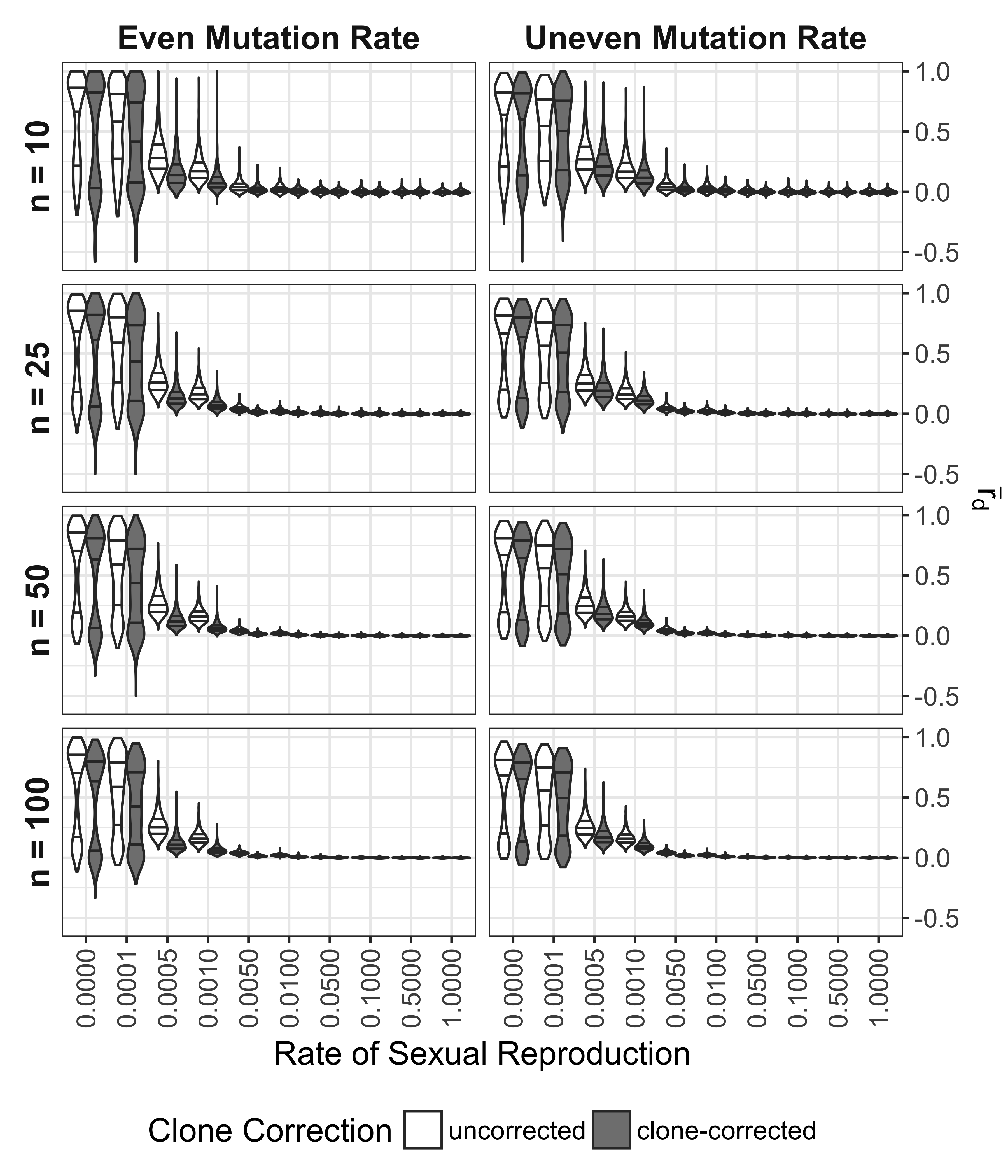
$Effect of rate of sexual reproduction, sample size (n), mutation rate, and clone-correction on $\bar{r}_d$ for microsatellite data. Violin plots represent data sets simulated with even and uneven mutation rates over 20 and 21 loci, respectively (columns) and sub-sampled in four different population sizes (rows). Color indicates whether or not the calculations were performed on whole or clone-corrected data sets. Each violin plot contains 1000 unique data sets. Black lines in violins mark the 25, 50, and 75th percentile.$

Figure 5.1: Effect of rate of sexual reproduction, sample size (n), mutation rate, and clone-correction on $\bar{r}_d$ for microsatellite data. Violin plots represent data sets simulated with even and uneven mutation rates over 20 and 21 loci, respectively (columns) and sub-sampled in four different population sizes (rows). Color indicates whether or not the calculations were performed on whole or clone-corrected data sets. Each violin plot contains 1000 unique data sets. Black lines in violins mark the 25, 50, and 75th percentile.

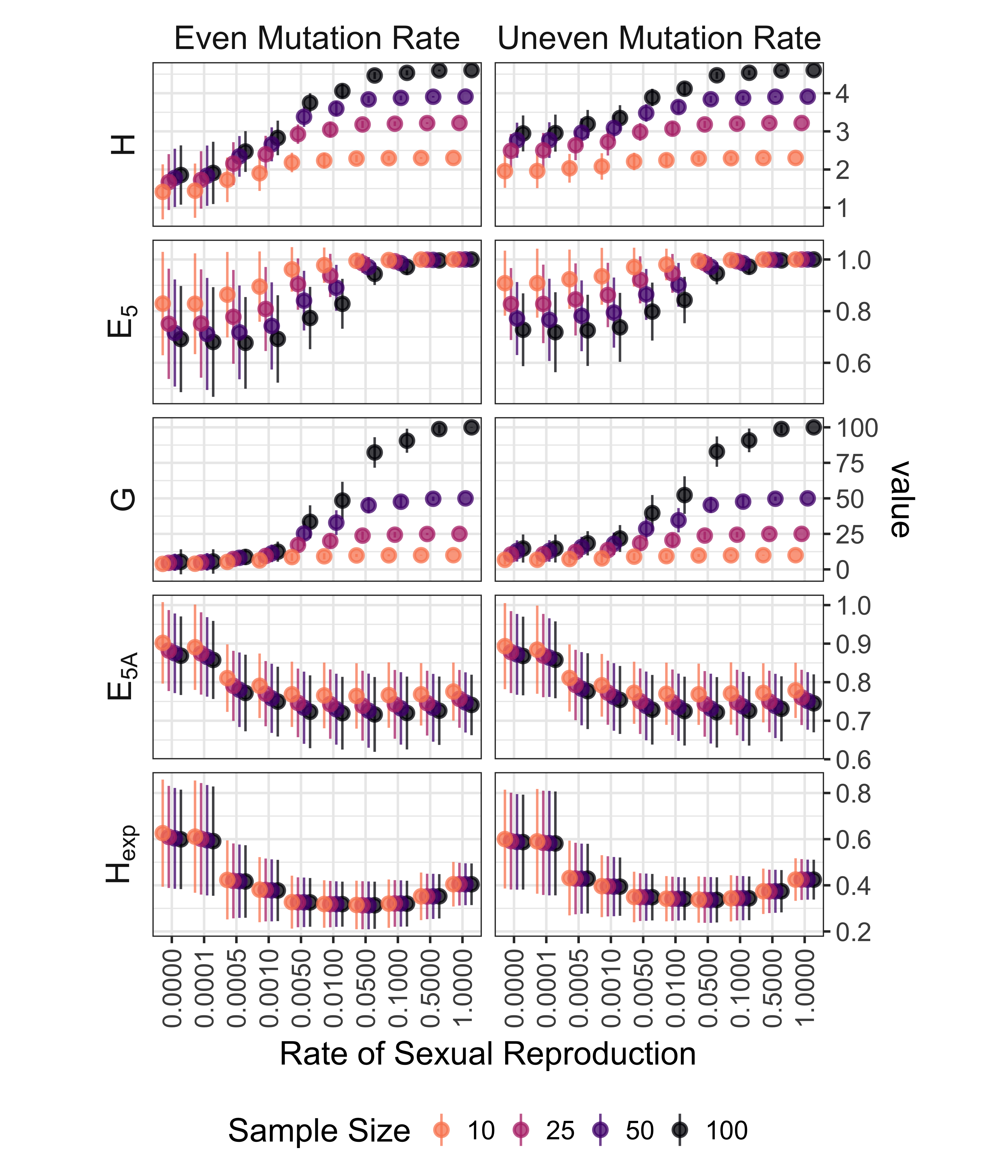
$Effect rate of sexual reproduction and sample size (n) on genotypic and allelic diversity for microsatellite data. Genotypic diversity: H = Shannon-Wiener index, $E_5$ = evenness, G = Stoddart and Taylor's index. Allelic Diversity: $E_{5A}$ = allelic evenness, $H_{exp}$ = Nei's expected heterozygosity (gene diversity). Allelic diversity estimates calculated for clone-corrected data. Points indicate means and lines extend to to standard deviations on either side of the mean. Color/shading indicates sample size. Vertical axis on different scales.$

Figure 5.2: Effect rate of sexual reproduction and sample size (n) on genotypic and allelic diversity for microsatellite data. Genotypic diversity: H = Shannon-Wiener index, $E_5$ = evenness, G = Stoddart and Taylor’s index. Allelic Diversity: $E_{5A}$ = allelic evenness, $H_{exp}$ = Nei’s expected heterozygosity (gene diversity). Allelic diversity estimates calculated for clone-corrected data. Points indicate means and lines extend to to standard deviations on either side of the mean. Color/shading indicates sample size. Vertical axis on different scales.

Effect of rate of sexual reproduction, sample size (n), mutation rate,
and clone-correction on the power of permutation analysis for microsatellite
data. Power (true positive rate) is on the vertical axis. Values are shown for p
= 0.01. Plots are arranged in a grid with clone-correction in rows and mutation
rate in columns. Color indicates sample size.

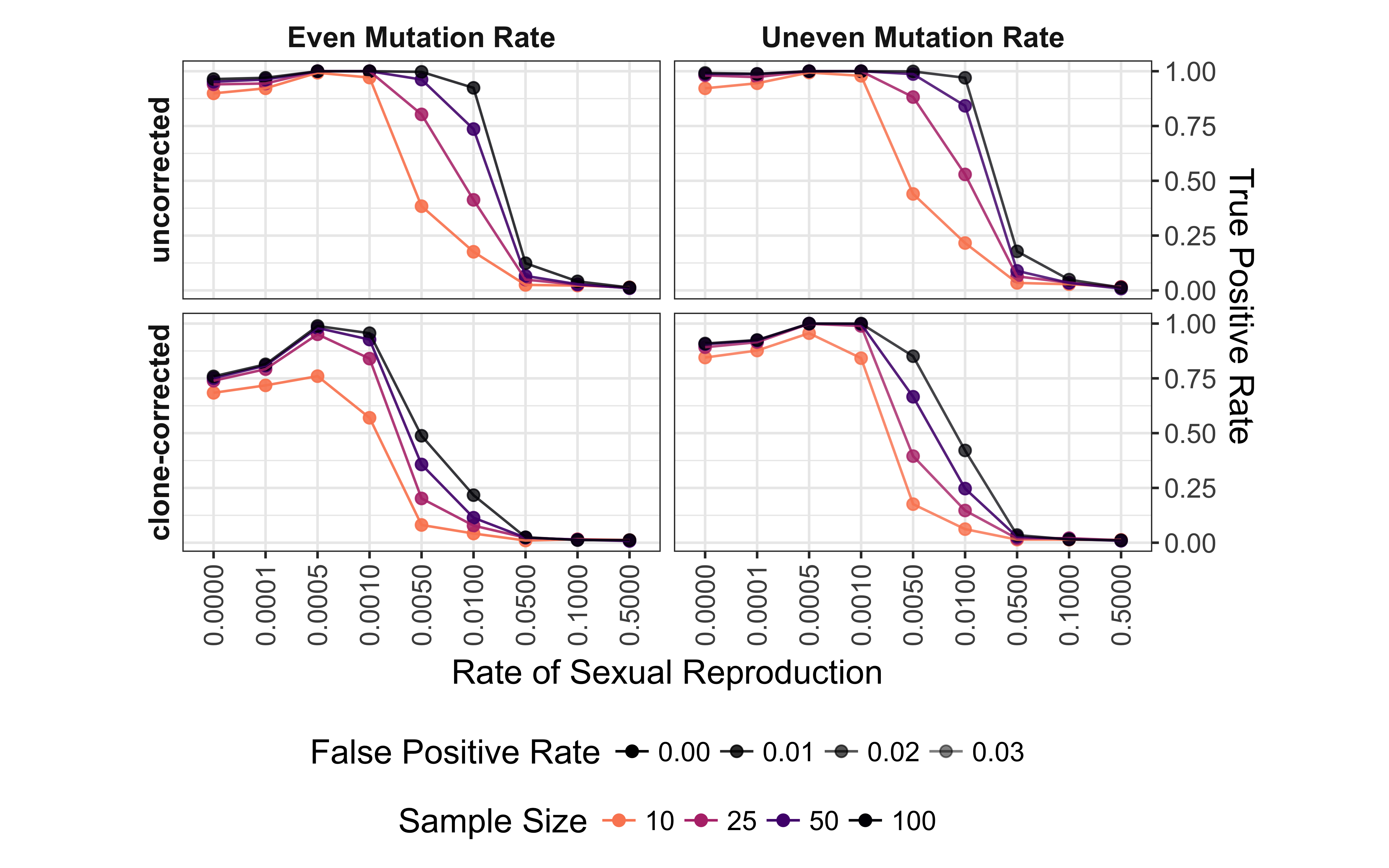
Figure 5.3: Effect of rate of sexual reproduction, sample size (n), mutation rate, and clone-correction on the power of permutation analysis for microsatellite data. Power (true positive rate) is on the vertical axis. Values are shown for p = 0.01. Plots are arranged in a grid with clone-correction in rows and mutation rate in columns. Color indicates sample size.

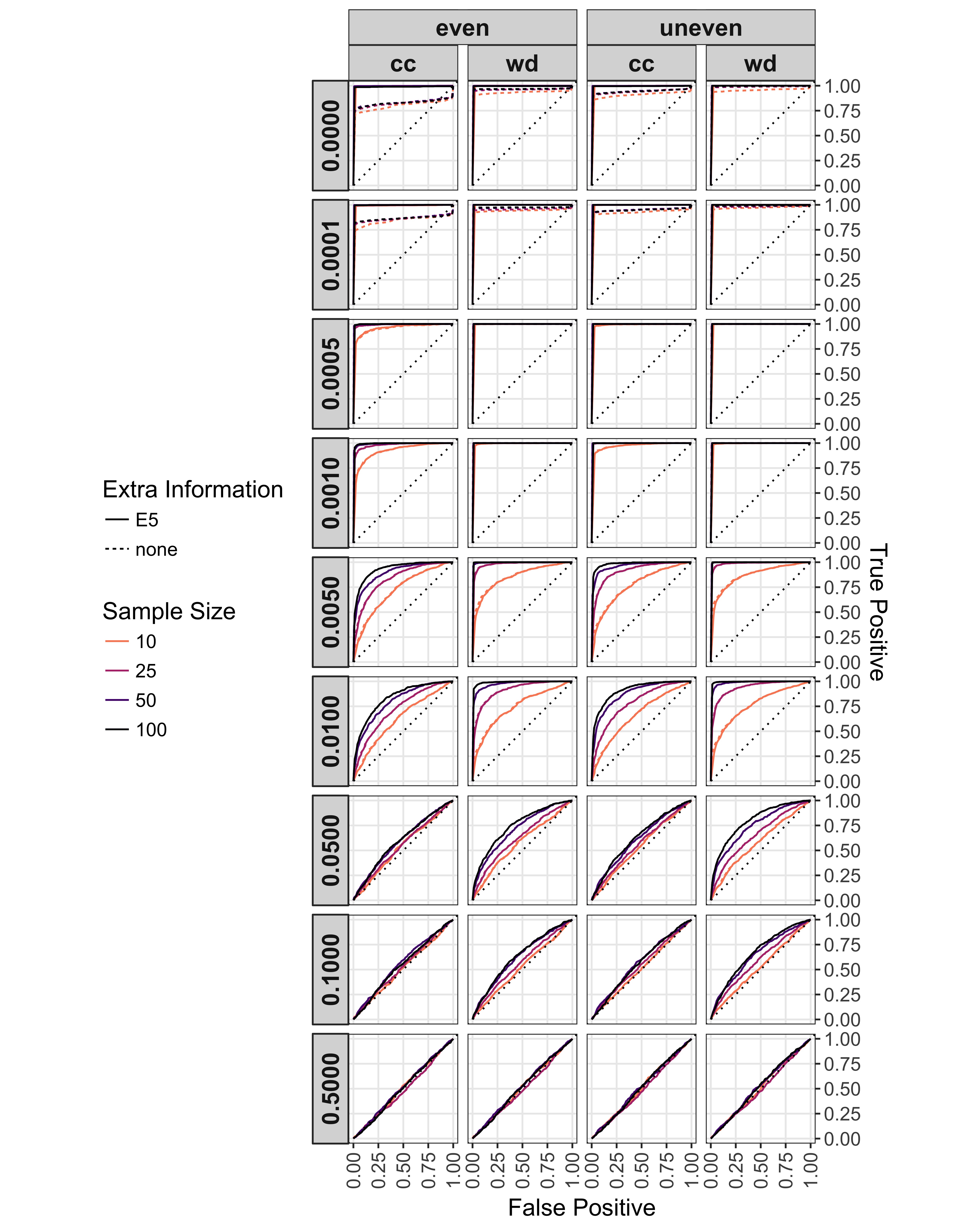
$Effect of rate of sexual reproduction, sample size (n), mutation rate, clone-correction, and $E_{5A}$ augmentation on ROC analysis of $\bar{r}_d$. Rate of sexual reproduction arranged in rows. Clone corrected (cc) and whole (wd) data sets with even and uneven mutation rates arranged in columns. Line type indicates the use of $E_{5A}$ > 0.85 to augment the analysis. Line shade indicates sample size. A dotted line of unity is shown in each plot. Each ROC curve is calculated over 100 values of $\alpha$ from 0 to 1.$

Figure 5.4: Effect of rate of sexual reproduction, sample size (n), mutation rate, clone-correction, and $E_{5A}$ augmentation on ROC analysis of $\bar{r}_d$. Rate of sexual reproduction arranged in rows. Clone corrected (cc) and whole (wd) data sets with even and uneven mutation rates arranged in columns. Line type indicates the use of $E_{5A}$ > 0.85 to augment the analysis. Line shade indicates sample size. A dotted line of unity is shown in each plot. Each ROC curve is calculated over 100 values of $\alpha$ from 0 to 1.

The ROC and AURC analyses showed a steady decrease in the ability to detect non- random mating with increasing levels of sexual reproduction, mainly due to a loss in sensitivity with increasing levels of $\alpha$ (Fig. 5.4, 5.5). As seen in the power analysis (Fig. 5.3), clone correction consistently appears to lower the power to detect linkage based on the AURC. For all scenarios, the diagnostic power of $\bar{r}_d$ to detect non-random mating is no better than random at rates of sexual reproduction greater than 10%.

A three-way ANOVA adds support for the hypothesis that clone correction significantly affects the diagnostic power of $\bar{r}_d$ (Fig. 5.6, Table 5.2). While there are no significant effects at 50% sex, clone correction, mutation rate, and sample size all have a significant effect on $\bar{r}_d$’s diagnostic properties. At low levels of sex (< 1%), the interaction of clone correction and mutation rate shows a significant effect, which is not seen in the interaction of clone correction and sample size. Only at sex rates of 0.1% and 0.05% do we see significant effects across all interactions.

Effect of rate of sexual reproduction, sample size (n), mutation rate,
and clone-correction on area under the ROC curve. Box plots showing the
distribution of the AURC for each independent seed. Boxes span the interquartile
range (IQR) and the whiskers extend to 1.5 * IQR. An AURC of 1 indicates a
perfect classifier, while an AURC of 0.5 indicates the classifier is no better
than a random guess. Any values below 0.5 (shaded in grey) are considered worse
than random.

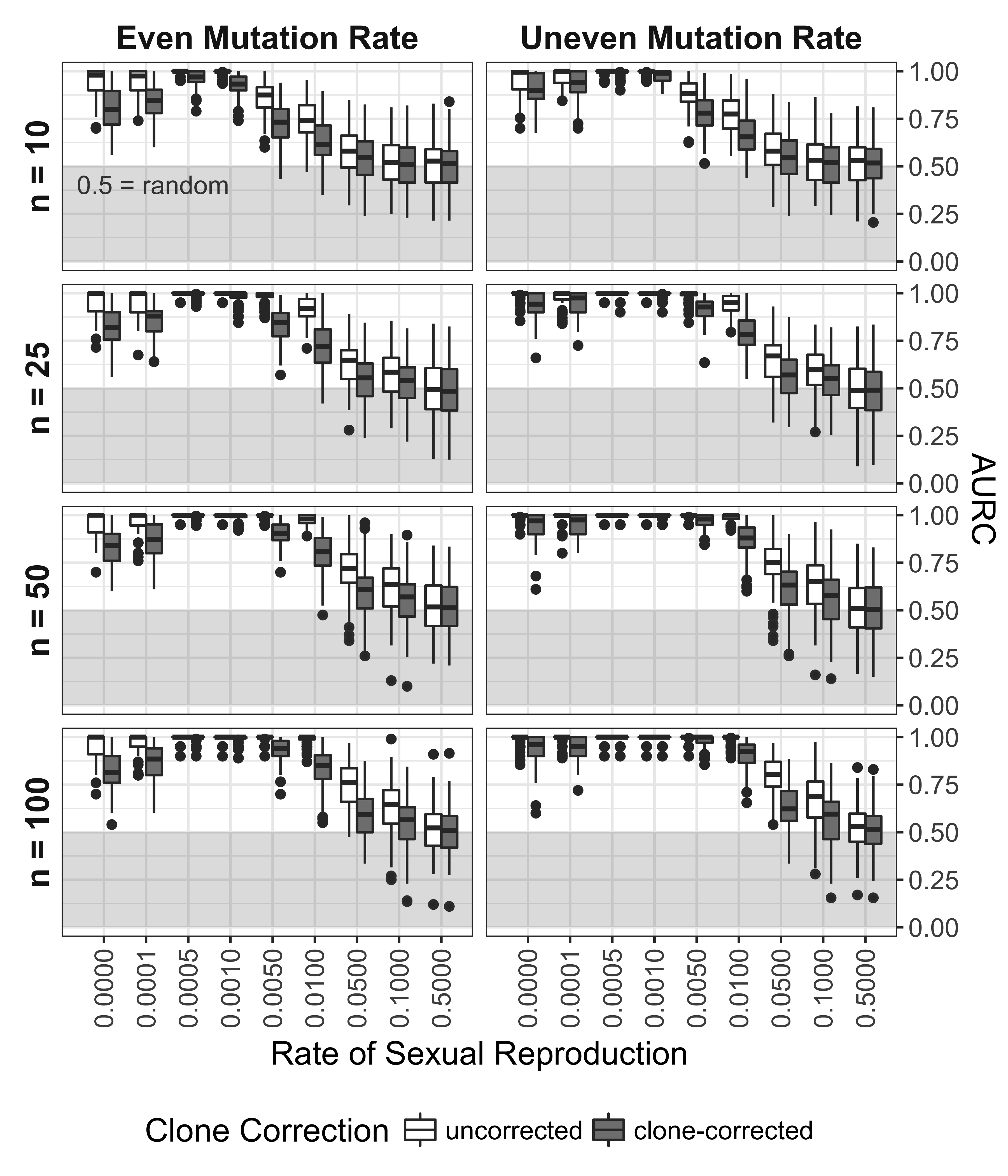
Figure 5.5: Effect of rate of sexual reproduction, sample size (n), mutation rate, and clone-correction on area under the ROC curve. Box plots showing the distribution of the AURC for each independent seed. Boxes span the interquartile range (IQR) and the whiskers extend to 1.5 * IQR. An AURC of 1 indicates a perfect classifier, while an AURC of 0.5 indicates the classifier is no better than a random guess. Any values below 0.5 (shaded in grey) are considered worse than random.

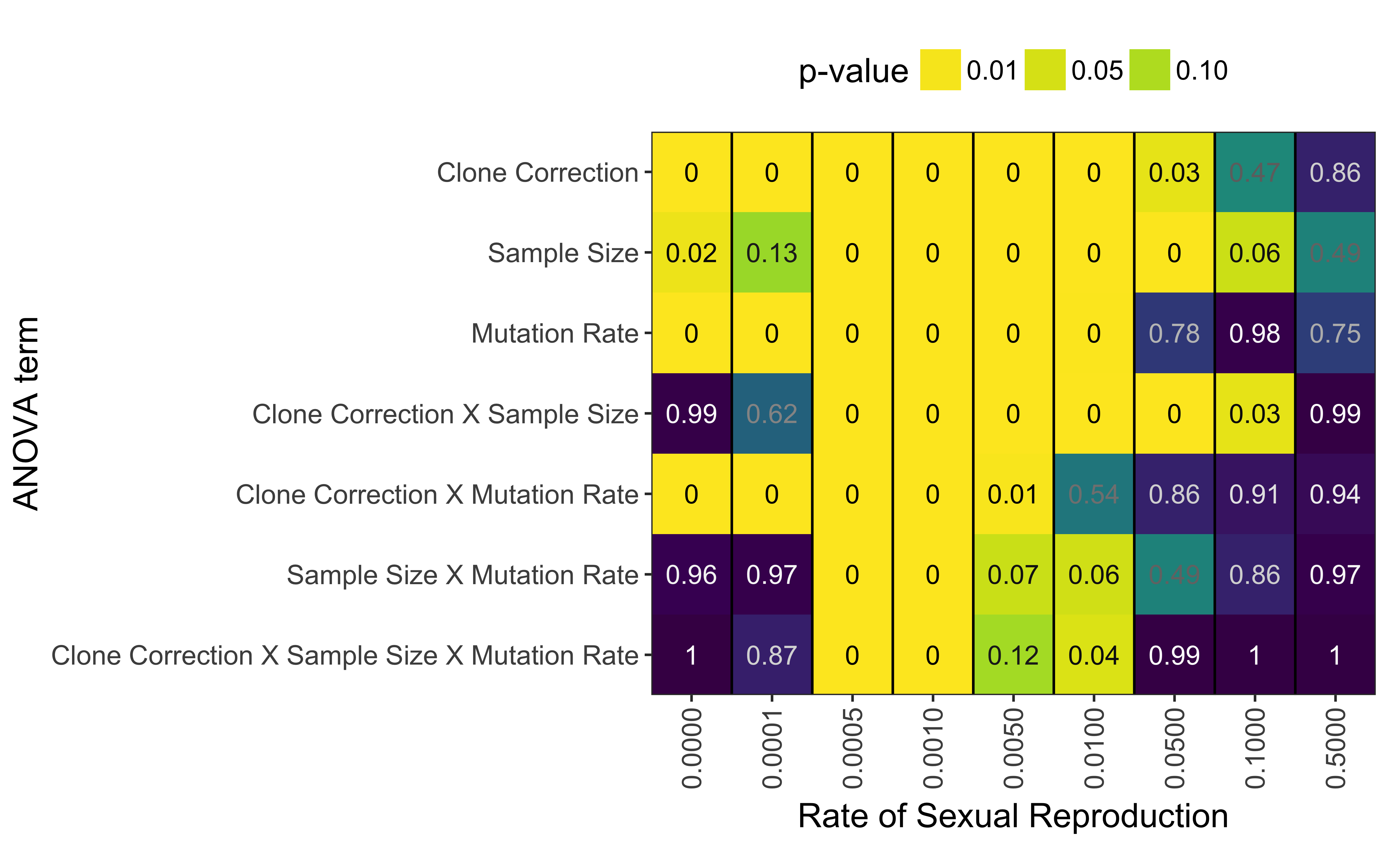
$P-values from ANOVA analysis assessing AURC distributions with the model $AURC \sim Clone Correction \times Sample Size \times Mutation Rate$ for each rate of sexual reproduction, separately.$

Figure 5.6: P-values from ANOVA analysis assessing AURC distributions with the model $AURC \sim Clone Correction \times Sample Size \times Mutation Rate$ for each rate of sexual reproduction, separately.

Table 5.2: ANOVA table comparing the model $AURC \sim Clone Correction \times Sample Size \times Mutation Rate$ for each rate of sexual reproduction separately. Columns: sexrate = rate of sexual reproduction, term = ANOVA term, sumsq = sum of squares, df = degrees of freedom, statistic = F statistic, p.value = p-value, Terms are as follows: CC = Clone Correction, SS = Sample Size, MR = Mutation Rate.
sexrate	term	sumsq	df	statistic	p.value
0.0000	(Intercept)	63.936	1	10569.674	0.000
	CC	0.855	1	141.309	0.000
	SS	0.060	3	3.289	0.020
	MR	0.556	1	91.913	0.000
	CC X SS	0.001	3	0.049	0.985
	CC X MR	0.174	1	28.747	0.000
	SS X MR	0.002	3	0.100	0.960
	CC X SS X MR	0.000	3	0.006	0.999
	Residuals	9.582	1584	NA	NA
0.0001	(Intercept)	70.972	1	14652.094	0.000
	CC	0.496	1	102.400	0.000
	SS	0.027	3	1.886	0.130
	MR	0.340	1	70.257	0.000
	CC X SS	0.009	3	0.596	0.617
	CC X MR	0.076	1	15.698	0.000
	SS X MR	0.001	3	0.077	0.972
	CC X SS X MR	0.003	3	0.241	0.868
	Residuals	7.673	1584	NA	NA
0.0005	(Intercept)	91.939	1	245382.751	0.000
	CC	0.072	1	191.181	0.000
	SS	0.089	3	78.753	0.000
	MR	0.050	1	132.414	0.000
	CC X SS	0.047	3	42.205	0.000
	CC X MR	0.027	1	72.663	0.000
	SS X MR	0.035	3	31.105	0.000
	CC X SS X MR	0.018	3	15.818	0.000
	Residuals	0.593	1584	NA	NA
0.0010	(Intercept)	86.202	1	157278.033	0.000
	CC	0.224	1	408.905	0.000
	SS	0.269	3	163.853	0.000
	MR	0.113	1	206.697	0.000
	CC X SS	0.135	3	82.053	0.000
	CC X MR	0.060	1	109.071	0.000
	SS X MR	0.067	3	40.994	0.000
	CC X SS X MR	0.034	3	20.426	0.000
	Residuals	0.868	1584	NA	NA
0.0050	(Intercept)	52.266	1	14127.572	0.000
	CC	0.936	1	253.111	0.000
	SS	2.592	3	233.531	0.000
	MR	0.138	1	37.393	0.000
	CC X SS	0.234	3	21.126	0.000
	CC X MR	0.028	1	7.675	0.006
	SS X MR	0.026	3	2.385	0.068
	CC X SS X MR	0.022	3	1.974	0.116
	Residuals	5.860	1584	NA	NA
0.0100	(Intercept)	39.376	1	5724.212	0.000
	CC	0.686	1	99.672	0.000
	SS	2.455	3	118.955	0.000
	MR	0.068	1	9.817	0.002
	CC X SS	0.173	3	8.380	0.000
	CC X MR	0.003	1	0.378	0.539
	SS X MR	0.051	3	2.488	0.059
	CC X SS X MR	0.056	3	2.720	0.043
	Residuals	10.896	1584	NA	NA
0.0500	(Intercept)	28.671	1	1903.303	0.000
	CC	0.072	1	4.806	0.029
	SS	0.239	3	5.293	0.001
	MR	0.001	1	0.080	0.778
	CC X SS	0.391	3	8.646	0.000
	CC X MR	0.000	1	0.032	0.858
	SS X MR	0.037	3	0.809	0.489
	CC X SS X MR	0.001	3	0.028	0.994
	Residuals	23.861	1584	NA	NA
0.1000	(Intercept)	26.010	1	1441.495	0.000
	CC	0.009	1	0.524	0.469
	SS	0.131	3	2.419	0.065
	MR	0.000	1	0.001	0.979
	CC X SS	0.162	3	2.984	0.030
	CC X MR	0.000	1	0.013	0.908
	SS X MR	0.014	3	0.256	0.857
	CC X SS X MR	0.001	3	0.015	0.998
	Residuals	28.581	1584	NA	NA
0.5000	(Intercept)	25.669	1	1489.342	0.000
	CC	0.001	1	0.033	0.857
	SS	0.042	3	0.806	0.491
	MR	0.002	1	0.099	0.753
	CC X SS	0.001	3	0.025	0.995
	CC X MR	0.000	1	0.006	0.939
	SS X MR	0.004	3	0.076	0.973
	CC X SS X MR	0.001	3	0.011	0.998
	Residuals	27.301	1584	NA	NA

5.4.2 Negative Values of $\bar{r}_d$ in Clonal Populations Correlated With Low Allelic Diversity

When using the criterion of $E_{5A} \geq 0.85$ to augment the criteria for the ROC analysis, we found that the power to detect non-random mating increased significantly whereas the false positive rate appeared to only increase with low sample sizes (Fig. 5.7, 5.8). Analyzing the distributions of the AURC with ANOVA, we found that the most consistently significant effect found was that of sample size (Fig. 5.9, Tab. 5.3) (albeit much like Fig. 5.6, all effects and interactions were significant for 0.1% and 0.05% sex).

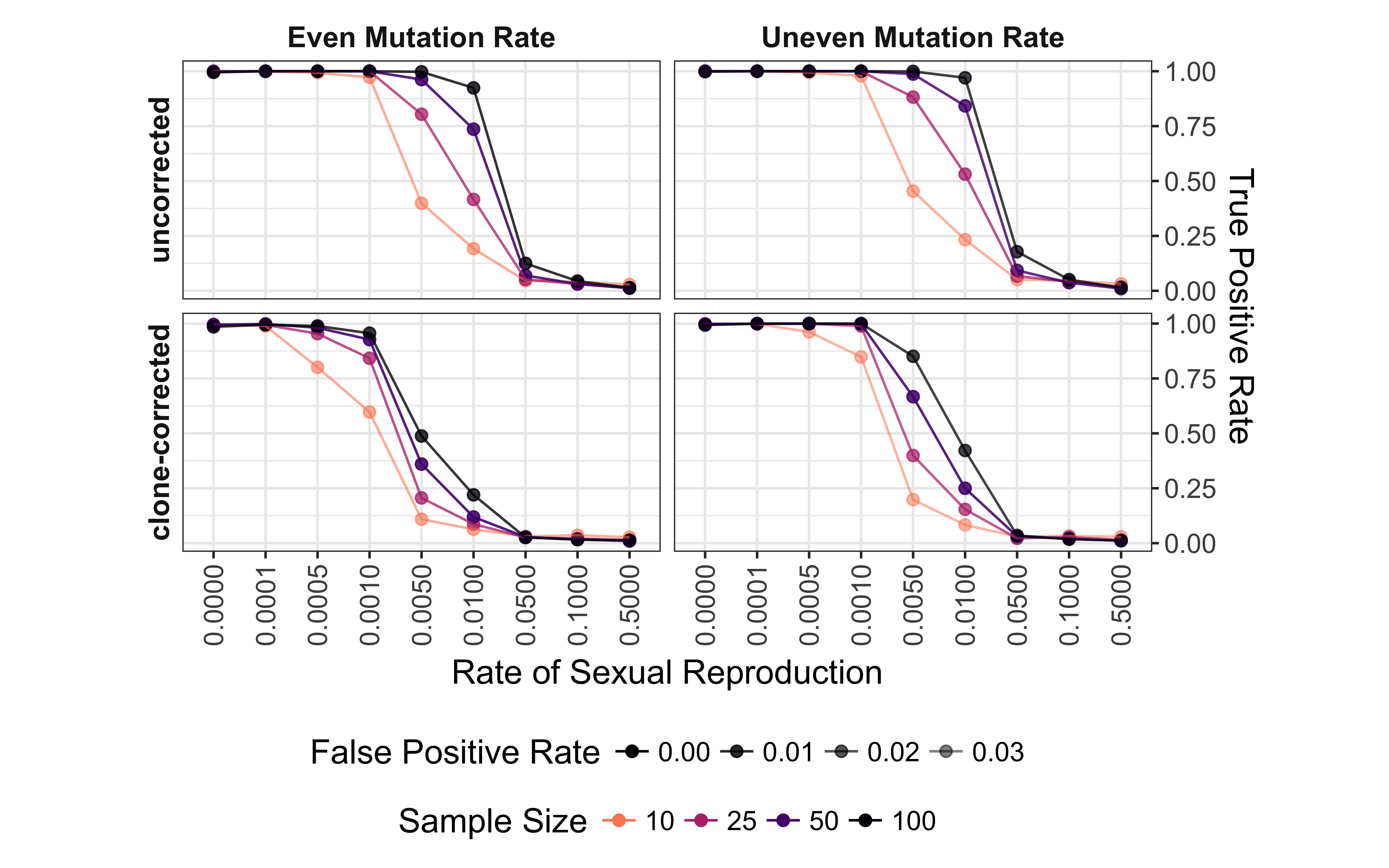
$Effect of rate of sexual reproduction, sample size (n), mutation rate, and clone-correction on the power of permutation analysis for microsatellite data taking into account allelic evenness. Plots are arranged in a grid with clone-correction in rows and mutation rate in columns. Values are shown for $\alpha$ = 0.01 and $E_{5A} \geq 0.85$$

Figure 5.7: Effect of rate of sexual reproduction, sample size (n), mutation rate, and clone-correction on the power of permutation analysis for microsatellite data taking into account allelic evenness. Plots are arranged in a grid with clone-correction in rows and mutation rate in columns. Values are shown for $\alpha$ = 0.01 and $E_{5A} \geq 0.85$

Effect of rate of sexual reproduction, sample size (n), mutation rate,
and clone-correction on area under the ROC curve taking into account allelic
evenness. Box plots showing the distribution of the area under the ROC Curve for
each independent seed. Boxes span the interquartile range (IQR) and the whiskers
extend to 1.5 * IQR. An AURC of 1 indicates a perfect classifier, while an AURC
of 0.5 indicates the classifier is no better than a random guess. Any values
below 0.5 (shaded in grey) is considered worse than random.

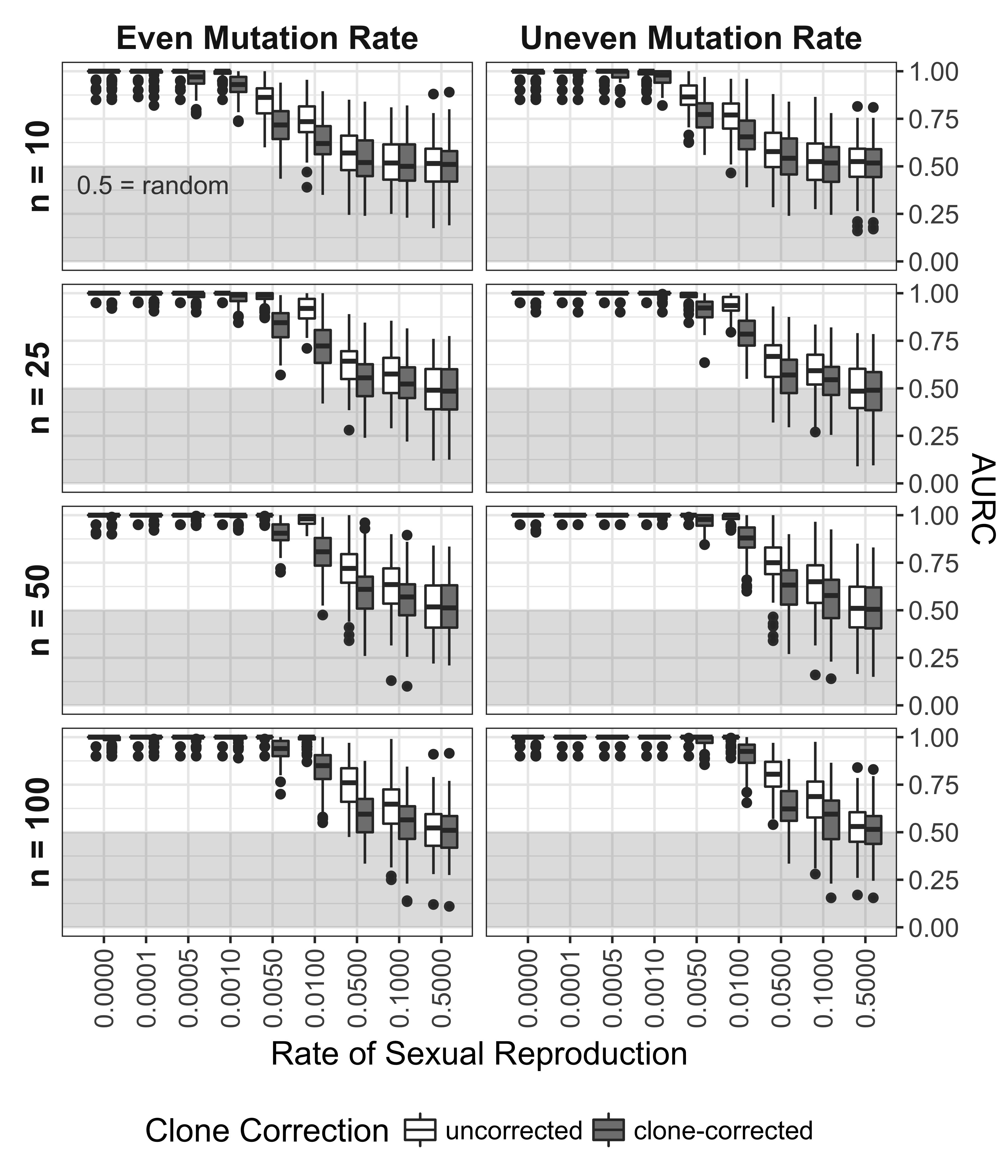
Figure 5.8: Effect of rate of sexual reproduction, sample size (n), mutation rate, and clone-correction on area under the ROC curve taking into account allelic evenness. Box plots showing the distribution of the area under the ROC Curve for each independent seed. Boxes span the interquartile range (IQR) and the whiskers extend to 1.5 * IQR. An AURC of 1 indicates a perfect classifier, while an AURC of 0.5 indicates the classifier is no better than a random guess. Any values below 0.5 (shaded in grey) is considered worse than random.

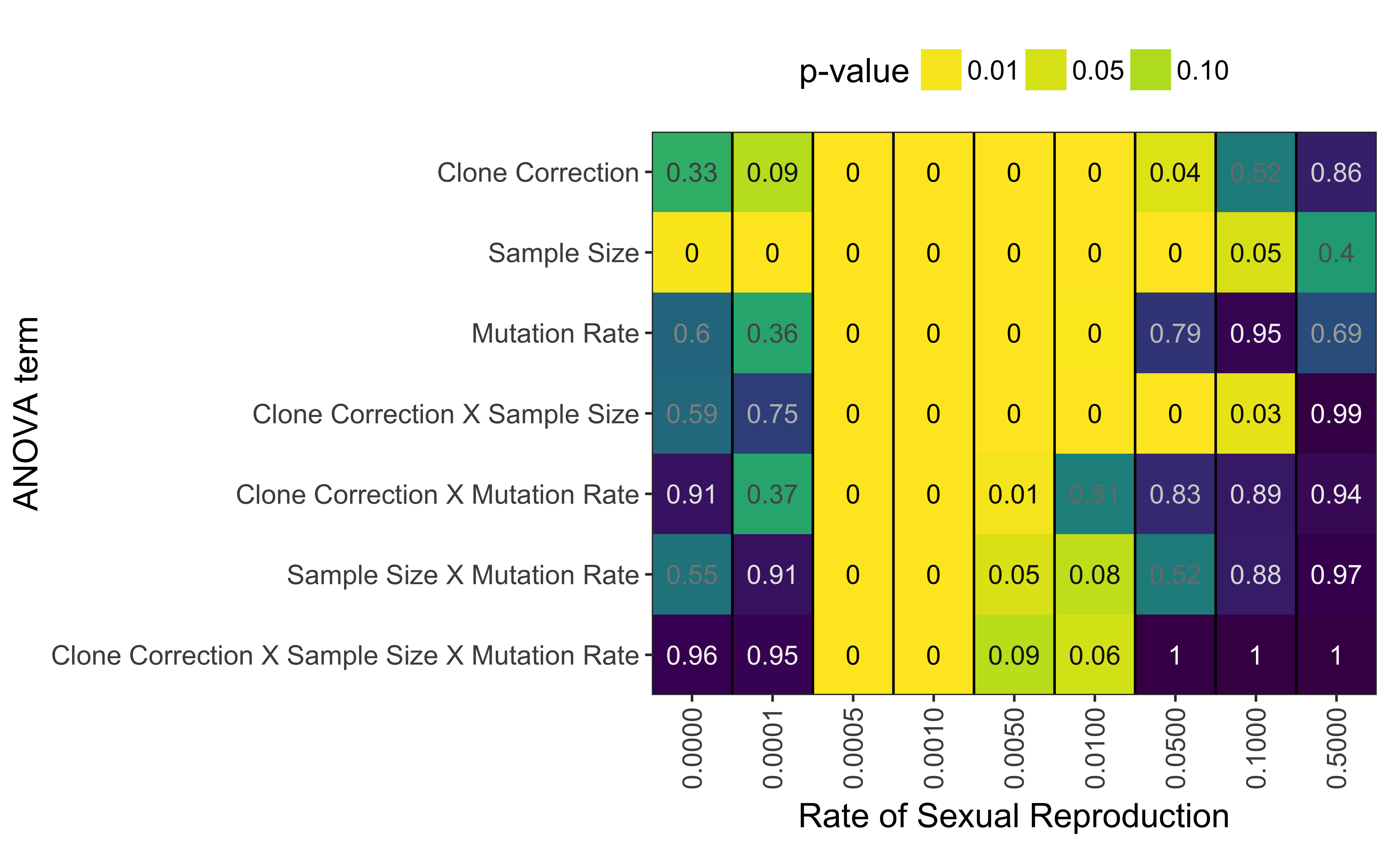
$P-values from ANOVA analysis on AURC distributions with the model $AURC \sim Clone Correction \times Sample Size \times Mutation Rate$ for each rate of sexual reproduction separately taking into account allelic evenness. P-values are represented both as colors and numbers.$

Figure 5.9: P-values from ANOVA analysis on AURC distributions with the model $AURC \sim Clone Correction \times Sample Size \times Mutation Rate$ for each rate of sexual reproduction separately taking into account allelic evenness. P-values are represented both as colors and numbers.

Table 5.3: ANOVA table comparing the model $AURC \sim Clone Correction \times Sample Size \times Mutation Rate$ for each rate of sexual reproduction separately. This table generated with the allelic evenness correction. Columns: sexrate = rate of sexual reproduction, term = ANOVA term, sumsq = sum of squares, df = degrees of freedom, statistic = F statistic, p.value = p-value, Terms are as follows: CC = Clone Correction, SS = Sample Size, MR = Mutation Rate.
sexrate	term	sumsq	df	statistic	p.value
0.0000	(Intercept)	96.914	1	169384.022	0.000
	CC	0.001	1	0.952	0.329
	SS	0.007	3	4.365	0.005
	MR	0.000	1	0.268	0.605
	CC X SS	0.001	3	0.638	0.591
	CC X MR	0.000	1	0.013	0.908
	SS X MR	0.001	3	0.704	0.550
	CC X SS X MR	0.000	3	0.104	0.958
	Residuals	0.906	1584	NA	NA
0.0001	(Intercept)	96.531	1	202595.988	0.000
	CC	0.001	1	2.838	0.092
	SS	0.009	3	6.345	0.000
	MR	0.000	1	0.823	0.365
	CC X SS	0.001	3	0.404	0.750
	CC X MR	0.000	1	0.819	0.366
	SS X MR	0.000	3	0.178	0.911
	CC X SS X MR	0.000	3	0.112	0.953
	Residuals	0.755	1584	NA	NA
0.0005	(Intercept)	91.136	1	158601.676	0.000
	CC	0.051	1	89.102	0.000
	SS	0.106	3	61.325	0.000
	MR	0.036	1	61.799	0.000
	CC X SS	0.033	3	19.237	0.000
	CC X MR	0.019	1	33.262	0.000
	SS X MR	0.024	3	14.139	0.000
	CC X SS X MR	0.012	3	7.046	0.000
	Residuals	0.910	1584	NA	NA
0.0010	(Intercept)	84.686	1	113261.634	0.000
	CC	0.211	1	282.532	0.000
	SS	0.339	3	151.115	0.000
	MR	0.103	1	137.833	0.000
	CC X SS	0.126	3	56.324	0.000
	CC X MR	0.053	1	71.367	0.000
	SS X MR	0.061	3	26.976	0.000
	CC X SS X MR	0.030	3	13.161	0.000
	Residuals	1.184	1584	NA	NA
0.0050	(Intercept)	51.087	1	13448.247	0.000
	CC	0.888	1	233.702	0.000
	SS	2.812	3	246.742	0.000
	MR	0.127	1	33.301	0.000
	CC X SS	0.226	3	19.851	0.000
	CC X MR	0.024	1	6.284	0.012
	SS X MR	0.031	3	2.682	0.045
	CC X SS X MR	0.025	3	2.186	0.088
	Residuals	6.017	1584	NA	NA
0.0100	(Intercept)	38.906	1	5499.579	0.000
	CC	0.634	1	89.610	0.000
	SS	2.558	3	120.521	0.000
	MR	0.070	1	9.912	0.002
	CC X SS	0.182	3	8.581	0.000
	CC X MR	0.003	1	0.443	0.506
	SS X MR	0.048	3	2.270	0.079
	CC X SS X MR	0.054	3	2.531	0.056
	Residuals	11.206	1584	NA	NA
0.0500	(Intercept)	28.404	1	1861.840	0.000
	CC	0.064	1	4.165	0.041
	SS	0.274	3	5.996	0.000
	MR	0.001	1	0.072	0.788
	CC X SS	0.401	3	8.760	0.000
	CC X MR	0.001	1	0.049	0.825
	SS X MR	0.035	3	0.759	0.517
	CC X SS X MR	0.001	3	0.020	0.996
	Residuals	24.165	1584	NA	NA
0.1000	(Intercept)	25.985	1	1413.238	0.000
	CC	0.008	1	0.422	0.516
	SS	0.145	3	2.632	0.049
	MR	0.000	1	0.004	0.952
	CC X SS	0.164	3	2.974	0.031
	CC X MR	0.000	1	0.019	0.891
	SS X MR	0.013	3	0.229	0.876
	CC X SS X MR	0.001	3	0.012	0.998
	Residuals	29.124	1584	NA	NA
0.5000	(Intercept)	25.366	1	1459.705	0.000
	CC	0.001	1	0.030	0.862
	SS	0.051	3	0.978	0.402
	MR	0.003	1	0.158	0.691
	CC X SS	0.001	3	0.026	0.994
	CC X MR	0.000	1	0.005	0.943
	SS X MR	0.004	3	0.078	0.972
	CC X SS X MR	0.001	3	0.010	0.999
	Residuals	27.526	1584	NA	NA

5.4.3 Power To Detect Clonal Reproduction in SNP Data

Because of the computational intensity of the simulations, we were only able to run 24 unique seeds over all rates of sexual reproduction with 10 replicates per seed. Due to an unexpected corner condition, some replicates failed to save, so we randomly sampled five replicates per seed per rate of sexual reproduction, giving us a total of 1,200 total populations for analysis.

Analysis of $\bar{r}_d$ for SNP data showed a similar pattern to the microsatellite data where clonal and nearly clonal (0.1% sexual reproduction) distributions of $\bar{r}_d$ were bimodal, but they did not have as many significantly negative values (Fig. 5.10). We observed that that none of the values of $\bar{r}_d$ for the sexual population reached zero. Increasing levels of missing data appeared to consistently decrease the value of $\bar{r}_d$ (5.11). This effect was magnified when missing data was treated as a new allele.

We initially randomized all loci independently to test for significant departures from random mating. Our results from that analysis showed p = 0.001 for all but two clonal data sets (data not shown). After shuffling each chromosome independently, we obtained significance values that better reflected our observations from the microsatellite data. Because of the dearth of significantly negative $\bar{r}_d$ values in clonal populations, the power of the index to detect clonal reproduction was greater, but at the cost of an increase in false positive rates (Fig. 5.12). An ANOVA analysis of the distributions of ROC over the 24 seeds showed significant differences for 0.5% to 10% sexual reproduction (Fig. 5.13, Tab. 5.4).

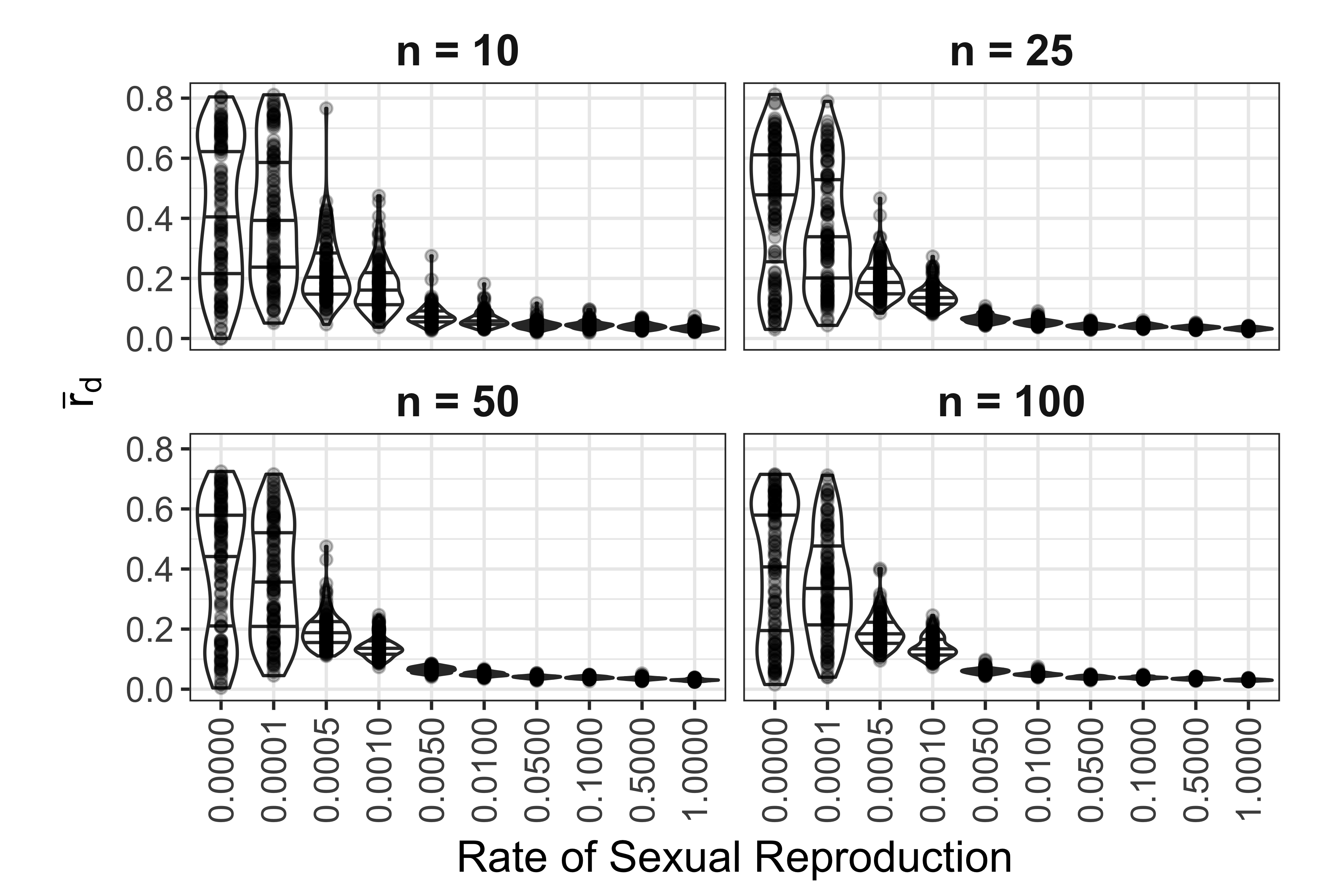
$Effect of rate of sexual reproduction and sample size (n) on $\bar{r}_d$ for SNP data. Each panel represents a different sample size. Each violin plot contains 120 unique data sets. Points represent observed values. Black lines in violins mark the 25, 50, and 75th percentile.$

Figure 5.10: Effect of rate of sexual reproduction and sample size (n) on $\bar{r}_d$ for SNP data. Each panel represents a different sample size. Each violin plot contains 120 unique data sets. Points represent observed values. Black lines in violins mark the 25, 50, and 75th percentile.

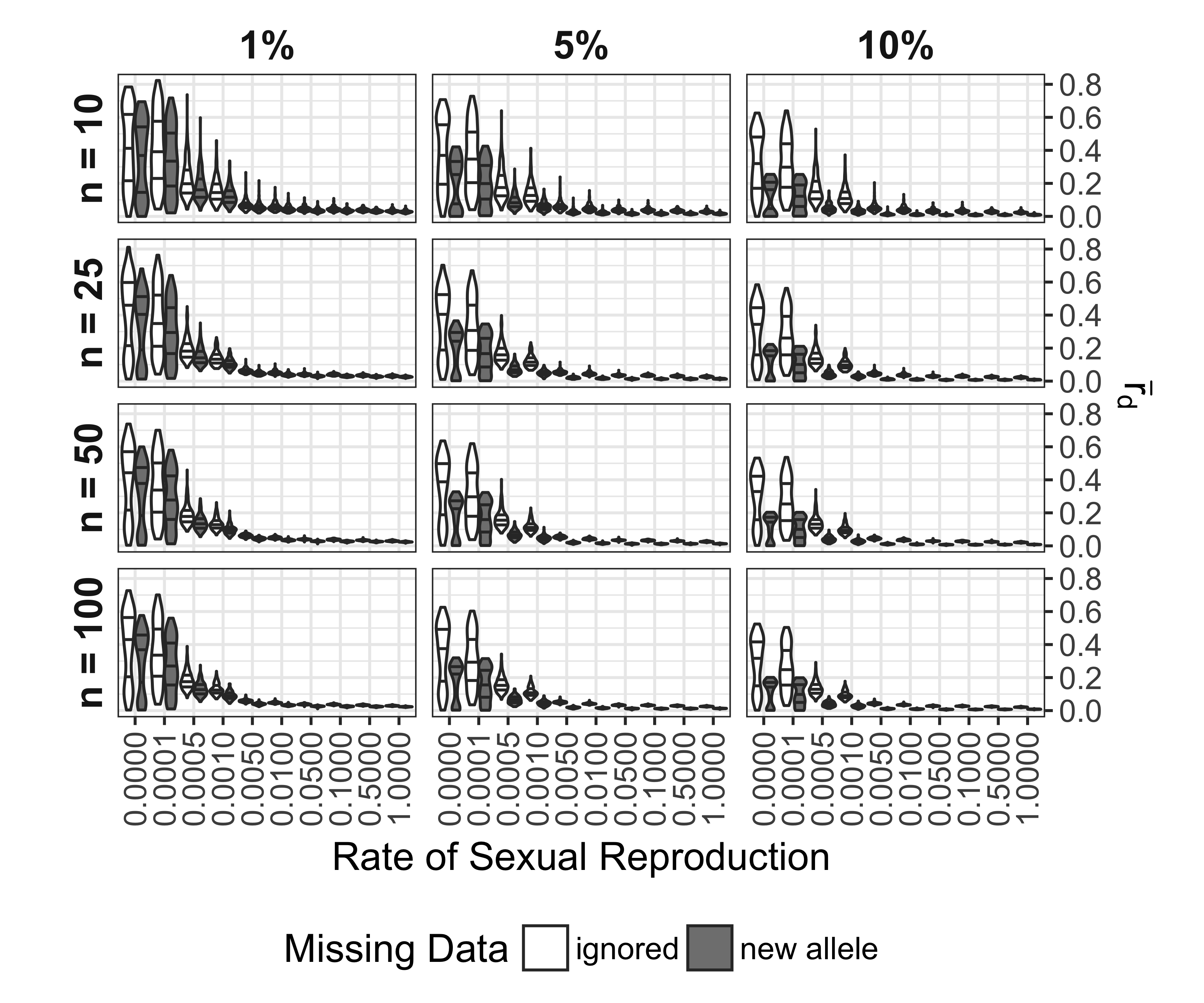
$Effect of rate of sexual reproduction, sample size (n), and missing data on $\bar{r}_d$ for SNP data. Panels are arranged horizontally with increasing rates of missing data from left to right and vertically with increasing sample size from top to bottom. Shading indicates whether or not missing data was ignored or treated as a new allele. Black lines mark the 25, 50, and 75th percentile. Each violin represents 120 values.$

Figure 5.11: Effect of rate of sexual reproduction, sample size (n), and missing data on $\bar{r}_d$ for SNP data. Panels are arranged horizontally with increasing rates of missing data from left to right and vertically with increasing sample size from top to bottom. Shading indicates whether or not missing data was ignored or treated as a new allele. Black lines mark the 25, 50, and 75th percentile. Each violin represents 120 values.

Effect of rate of sexual reproduction and sample size (n) the power to
detect non-random mating for SNP data. Color indicates sample size. False
positive rate is shown as increasing transparency. Data shown for both p = 0.01
and p = 0.05

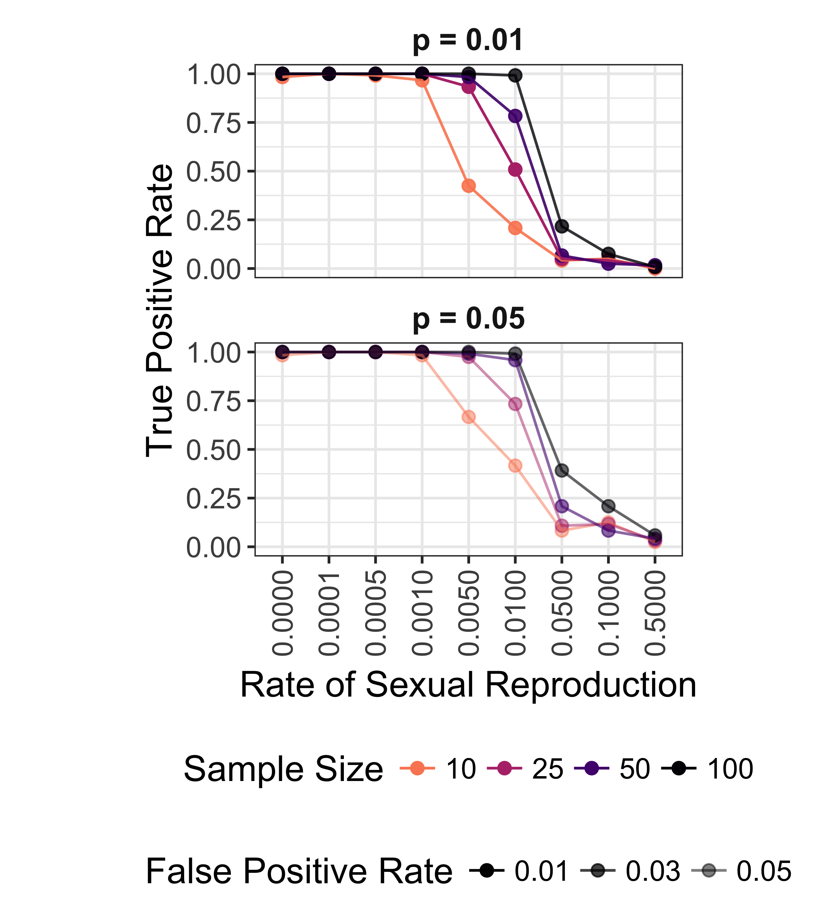
Figure 5.12: Effect of rate of sexual reproduction and sample size (n) the power to detect non-random mating for SNP data. Color indicates sample size. False positive rate is shown as increasing transparency. Data shown for both p = 0.01 and p = 0.05

Effect of rate of sexual reproduction and sample size (n) on area under
the ROC curve for SNP data. Each point represents AURC calculated with 10
populations total. 5 populations with a sex rate of 1.0 and 5 populations with a
sex rate specified on the horizontal axis.

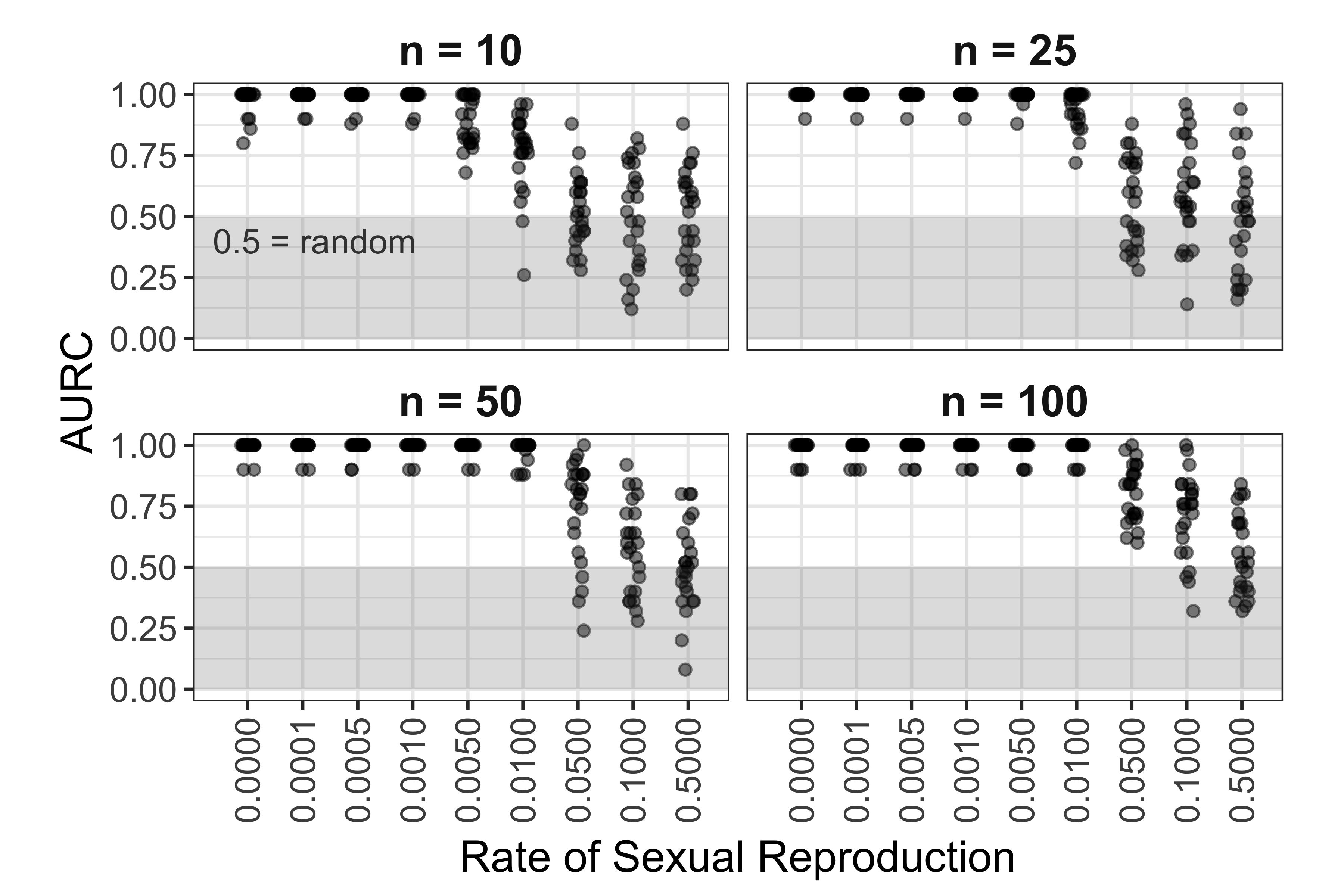
Figure 5.13: Effect of rate of sexual reproduction and sample size (n) on area under the ROC curve for SNP data. Each point represents AURC calculated with 10 populations total. 5 populations with a sex rate of 1.0 and 5 populations with a sex rate specified on the horizontal axis.

Table 5.4: ANOVA table comparing the model $AURC \sim Sample Size$ for each rate of sexual reproduction separately with SNP data. Columns: sexrate = rate of sexual reproduction, term = ANOVA term, sumsq = sum of squares, df = degrees of freedom, statistic = F statistic, p.value = p-value, Terms are as follows: SS = Sample Size.
sexrate	term	sumsq	df	statistic	p.value
0.0000	(Intercept)	22.932	1	17347.604	0.000
	SS	0.004	3	1.121	0.345
	Residuals	0.122	92	NA	NA
0.0001	(Intercept)	23.602	1	29949.701	0.000
	SS	0.001	3	0.352	0.787
	Residuals	0.072	92	NA	NA
0.0005	(Intercept)	23.562	1	28317.512	0.000
	SS	0.001	3	0.339	0.797
	Residuals	0.077	92	NA	NA
0.0010	(Intercept)	23.562	1	28317.512	0.000
	SS	0.001	3	0.339	0.797
	Residuals	0.077	92	NA	NA
0.0050	(Intercept)	19.117	1	6103.399	0.000
	SS	0.174	3	18.568	0.000
	Residuals	0.288	92	NA	NA
0.0100	(Intercept)	13.984	1	1590.890	0.000
	SS	0.806	3	30.552	0.000
	Residuals	0.809	92	NA	NA
0.0500	(Intercept)	6.510	1	232.786	0.000
	SS	1.340	3	15.972	0.000
	Residuals	2.573	92	NA	NA
0.1000	(Intercept)	5.920	1	155.018	0.000
	SS	0.575	3	5.023	0.003
	Residuals	3.514	92	NA	NA
0.5000	(Intercept)	6.161	1	169.859	0.000
	SS	0.059	3	0.542	0.655
	Residuals	3.337	92	NA	NA

5.4.4 Common Features of Microsatellite and SNP Markers

For both microsatellite and SNP data, as found in de Meeûs & Balloux (2004), large variances were observed with extremely low levels of sexual reproduction (Figs. 5.1, 5.10). The variances and means of $\bar{r}_d$ decrease with increasing levels of sexual reproduction. For low levels of sexual reproduction (< 0.01%), the distributions appeared bimodal. This feature appears in both the microsatellite and SNP data, but with microsatellite data, the lower part of the distribution extends into the negative values of $\bar{r}_d$, resulting in non-significant p-values, which occur when low allelic diversity is observed. Additionally, with larger sample sizes, the variances decrease (Fig. 5.1, 5.10) and the power to detect clonal reproduction increases (5.7, 5.12), suggesting that the behavior of the index is affected by sample size. Based on the power analysis, we observe that the critical point to detect clonal reproduction in a population is at a maximum of 1% sexual reproduction (Fig.5.3, 5.7, 5.12).

5.5 Discussion

Scientists have used the index of association to provide evidence for clonal reproduction in populations. The index of association measure the ratio of variance between observed and expected genetic distance and is a measure of linkage among markers (equation (5.1) ) (Brown et al., 1980; Smith et al., 1993). Agapow & Burt (2001) created a standardized version, $\bar{r}_d$, that resembles a correlation coefficient (equation (5.2)). De Meeûx & Balloux (2004) previously showed that very little sexual reproduction is required for $\bar{r}_d$ to reach values close to zero (e.g. the absence of linkage among markers). We confirmed that the power to detect clonal reproduction is greatly diminished after $\sim$ 1% sex in a population. We also provide novel insights into how $\bar{r}_d$ responds to marker type, sample size, mutation rate homogeneity, and clone-correction. We found that the power to detect significant departures of $\bar{r}_d$ from expected under random mating decreases with small sample sizes, and thus also decreases with clone-correction as sample size is by definition reduced when clone-correcting. More importantly, we found that linkage depends critically on allelic diversity at low levels of sexual reproduction (< 0.1%) as discussed below.

5.5.1 Clone Correction Increases False Negatives

While the presence of over-represented genotypes is often an indication of clonal reproduction, it does not explicitly rule out sexual reproduction (Smith et al., 1993; Taylor et al., 1999; Tibayrenc, 1996). This can happen in an ‘epidemic’ population structure where there is a sudden expansion of one genotype in an otherwise panmictic population (Smith et al., 1993). Thus, a common recommendation to researchers is to conduct analyses on both clone-corrected and uncorrected data with the expectation that this will reveal any underlying recombination (McDonald, 1997; Milgroom, 1996; Smith et al., 1993). When analyzing $\bar{r}_d$, common wisdom says that if the result is significant with and without clone-correction, then there is strong evidence for clonal reproduction. This technique was used by Goss et al. to support the hypothesis that South American populations of the potato late blight pathogen, Phytophthora infestans were reproducing clonally (2014). Our findings show that a non-significant value does not necessarily indicate the absence of clonal reproduction since the power to detect clonal reproduction consistently decreases with clone-correction(Fig. 5.5, 5.8). Our results confirm the concerns raised in Tibayrenc (1996) of the increase of false negatives due to clone- correction, further highlighting the fact that a failure to reject the null hypothesis of random mating does not necessarily mean that the population is randomly mating (Milgroom, 1996; Smith et al., 1993; Tibayrenc, 1996). Clone-correction thus should be interpreted carefully in light of the fact that clone-correction reduces sample size and power is significantly reduced with small sample sizes.

5.5.2 Mutation Rates and $\bar{r}_d$

We assessed the effect of uneven mutation rates across loci, because we had observed that a single, hyper-variable locus with 18 alleles was the driver for most of the diversity observed in a previous study on the population dynamics of Phytophthora ramorum in Curry County, OR (Kamvar et al. (2015 c), Supplementary Table S4). We hypothesized that the high variability would reduce linkage and thus, reduce the power of $\bar{r}_d$ to detect clonal reproduction. In contrast, we observed the opposite result; the power to detect clonal reproduction increased with the presence of a single, hyper-variable locus (Fig. 5.3, 5.4). This also appears to make the effects of clone-correction less severe. We believe that this is most likely due to the observed increase in genotypic diversity, which causes an increased sample size with clone-correction (Fig. 5.2).

5.5.3 Allelic Diversity Influences the value of $\bar{r}_d$ in Clonal Populations

A novel feature, not previously observed in de Meeûs & Balloux (2004), was the observation of negative values of $\bar{r}_d$ (Fig. 5.1). While positive values of $\bar{r}_d$ are easy to interpret (the observed variance is greater than expected, suggesting non-random mating), negative values are often simply considered to be evidence for random mating. Significantly (p = 1) negative values of $\bar{r}_d$ have been observed for pathogens that are well studied and known to be clonal such as the sudden oak death pathogen, Phytophthora ramorum (Kamvar et al. (2015 c), Supplementary Table S3) and the wheat stripe rust pathogen Puccinia graminis f.sp. tritici (Les Szabo, pers. comm.). A common pattern in all of these populations is that they all had values of $E_{5A}$ > 0.9 and, on average, fewer than 4 alleles per locus. This pattern of $E_{5A}$ is reflected in our simulations (Fig. 5.2). When we set a boundary condition for our power analysis based on evenness $\{p \leq \alpha \mid E_{5A} \geq 0.85\}$, we found that this reduced the number of false negatives without significantly contributing to the number of false positives (Fig. 5.7, 5.8). Levels of $E_{5A} > 0.85$ also had a low number of allelic states (data not shown), which indicates that the bimodal distribution of $\bar{r}_d$ for clonal populations is driven by allelic diversity. Thus, including allelic evenness can serve as a diagnostic parameter when interpreting linkage at low levels of sexual reproduction under conditions of low allelic diversity.

5.5.4 Linkage in SNP Data Increases $\bar{r}_d$ Unilaterally

The results we obtained from SNP data revealed almost no values of $\bar{r}_d$ at or below zero (Fig. 5.10). Testing for significance by shuffling data at each locus independently rendered all the values of $\bar{r}_d$ significant, regardless of rate of sexual reproduction. Only when we shuffled linkage groups were we able to obtain the same level of significance as compared to the microsatellite data. This indicates that it is possible to detect clonal reproduction with the same power as microsatellite markers even with physically linked markers. Great care, however must be taken to ensure that linkage blocks are shuffled together or that SNP markers are not linked before assessing significance of a value of $\bar{r}_d$. In contrast to the microsatellite data, sample size did not significantly affect power with high levels of clonal reproduction (Fig 5.13, Tab: 5.4).

5.5.5 Limitations of This Study

The scope of simulation studies are limited to the parameters used to generate the simulations. We do not know, for example, what effect selection, population subdivision, or polyploidy would have on inference of $\bar{r}_d$. While we were able to directly compare our populations with even and uneven mutation rates, because they both represent the exact same populations, we do not know if the effect we see is due to a higher average mutation rate, thus further study is needed to detect the effect of mutation rate in clonal populations. In contrast to de Meeûs & Balloux (2004), whereas their simulations had 99 alleles per locus, our simulations were designed with a small number of alleles per locus to better reflect microsatellite markers that would be selected for typical population genetic analyses. Because of this, there was a higher chance of homoplasy in our simulations. This, however was most likely beneficial to our analysis as our results show that low allelic diversity can lead to negative $\bar{r}_d$ values, which we have previously observed in data from purely clonal organisms.

5.5.6 Conclusions

The index of association is a valuable measure for lending support to the hypothesis of clonal reproduction in natural populations. We confirm that $\bar{r}_d$ can provide evidence for clonal reproduction when there is < 1% sexual reproduction within the population (de Meeûs & Balloux, 2004), but conclude that this inference is dependent on sample size and allelic diversity. Thus scientists should exercise caution when interpreting results from a clone-corrected data set. We found that this index is robust enough to detect the same level of clonal reproduction for SNP data, but results from permutation analyses may be misleading if linkage is present among markers.

References

Hartl, D. L., & Clark, A. G. (2007). Principles of population genetics. Sunderland, MA, USA: Sinauer Associates.

Nielsen, R., & Slatkin, M. (2013). An introduction to population genetics: Theory and applications. Sinauer Associates, Incorporated. Retrieved from http://books.google.com/books?id=Iy08kgEACAAJ

Milgroom, M. G. (1996). Recombination and the multilocus structure of fungal populations. Annual Review of Phytopathology, 34(1), 457–477.

Orive, M. E. (1993). Effective population size in organisms with complex life-histories. Theoretical Population Biology, 44(3), 316–340. https://doi.org/10.1006/tpbi.1993.1031

Heitman, J., Sun, S., & James, T. Y. (2012). Evolution of fungal sexual reproduction. Mycologia, 105(1), 1–27. https://doi.org/10.3852/12-253

Tibayrenc, M. (1996). Towards a unified evolutionary genetics of microorganisms. Annual Review of Microbiology, 50(1), 401–429. https://doi.org/10.1146/annurev.micro.50.1.401

de Meeûs, T., Lehmann, L., & Balloux, F. (2006). Molecular epidemiology of clonal diploids: A quick overview and a short DIY (do it yourself) notice. Infection, Genetics and Evolution, 6(2), 163–170. https://doi.org/10.1016/j.meegid.2005.02.004

Goss, E. M., Tabima, J. F., Cooke, D. E., Restrepo, S., Fry, W. E., Forbes, G. A., Fieland, V. J., Cardenas, M., & Grünwald, N. J. (2014). The Irish potato famine pathogen Phytophthora infestans originated in central Mexico rather than the Andes. Proceedings of the National Academy of Sciences, 111(24), 8791–8796.

Nieuwenhuis, B. P. S., & James, T. Y. (2016). The frequency of sex in fungi. Philosophical Transactions of the Royal Society B: Biological Sciences, 371(1706), 20150540. https://doi.org/10.1098/rstb.2015.0540

Smith, J. M., Smith, N. H., O’Rourke, M., & Spratt, B. G. (1993). How clonal are bacteria? Proceedings of the National Academy of Sciences, 90(10), 4384–4388. https://doi.org/10.1073/pnas.90.10.4384

Ali, S., Soubeyrand, S., Gladieux, P., Giraud, T., Leconte, M., Gautier, A., Mboup, M., Chen, W., Vallavieille-Pope, C., & Enjalbert, J. (2016). Cloncase: Estimation of sex frequency and effective population size by clonemate resampling in partially clonal organisms. Molecular Ecology Resources. https://doi.org/10.1111/1755-0998.12511

Balloux, F., Lehmann, L., & de Meeûs, T. (2003). The population genetics of clonal and partially clonal diploids. Genetics, 164(4), 1635–1644.

de Meeûs, T., & Balloux, F. (2004). Clonal reproduction and linkage disequilibrium in diploids: A simulation study. Infection, Genetics and Evolution, 4(4), 345–351. https://doi.org/10.1016/j.meegid.2004.05.002

Agapow, P.-M., & Burt, A. (2001). Indices of multilocus linkage disequilibrium. Molecular Ecology Notes, 1(1-2), 101–102. https://doi.org/10.1046/j.1471-8278.2000.00014.x

Brown, A., Feldman, M., & Nevo, E. (1980). Multilocus structure of natural populations of Hordeum spontaneum. Genetics, 96(2), 523–536. Retrieved from http://www.genetics.org/content/96/2/523.abstract

Haubold, B., Travisano, M., Rainey, P. B., & Hudson, R. R. (1998). Detecting linkage disequilibrium in bacterial populations. Genetics, 150(4), 1341–8.

Kamvar, Z. N., Tabima, J. F., & Grünwald, N. J. (2014b). Poppr : an R package for genetic analysis of populations with clonal, partially clonal, and/or sexual reproduction. PeerJ, 2, e281. https://doi.org/10.7717/peerj.281

Milgroom, M. G. (2015). Population biology of plant pathogens: Genetics, ecology, and evolution. 3340 Pilot Knob Road, St. Paul, MN 55121, USA: APS Press.

Prugnolle, F., & de Meeûs, T. (2010). Apparent high recombination rates in clonal parasitic organisms due to inappropriate sampling design. Heredity, 104(2), 135–140. https://doi.org/10.1038/hdy.2009.128

McDonald, B. A. (1997). The population genetics of fungi: tools and techniques. Phytopathology, 87(4), 448–453.

Davey, J. W., & Blaxter, M. L. (2010). RADSeq: next-generation population genetics. Briefings in Functional Genomics, 9(5-6), 416–423. https://doi.org/10.1093/bfgp/elq031

Davey, J. W., Hohenlohe, P. A., Etter, P. D., Boone, J. Q., Catchen, J. M., & Blaxter, M. L. (2011). Genome-wide genetic marker discovery and genotyping using next-generation sequencing. Nature Reviews Genetics, 12(7), 499–510. https://doi.org/10.1038/nrg3012

Elshire, R. J., Glaubitz, J. C., Sun, Q., Poland, J. A., Kawamoto, K., Buckler, E. S., & Mitchell, S. E. (2011). A robust, simple genotyping-by-sequencing (GBS) approach for high diversity species. PLoS ONE, 6(5), e19379. https://doi.org/10.1371/journal.pone.0019379

Mastretta-Yanes, A., Arrigo, N., Alvarez, N., Jorgensen, T. H., Piñero, D., & Emerson, B. C. (2014). Restriction site-associated DNA sequencing, genotyping error estimation and de novo assembly optimization for population genetic inference. Molecular Ecology Resources, 15(1), 28–41. https://doi.org/10.1111/1755-0998.12291

Kamvar, Z. N., Brooks, J. C., & Grünwald, N. J. (2015a). Novel R tools for analysis of genome-wide population genetic data with emphasis on clonality. Frontiers in Genetics, 6. https://doi.org/10.3389/fgene.2015.00208

R Core Team. (2016). R: A language and environment for statistical computing. Vienna, Austria: R Foundation for Statistical Computing. Retrieved from https://www.R-project.org/

Peng, B., & Amos, C. I. (2008). Forward-time simulations of non-random mating populations using simuPOP. Bioinformatics, 24(11), 1408–1409. https://doi.org/10.1093/bioinformatics/btn179

Lynch, M., Sung, W., Morris, K., Coffey, N., Landry, C. R., Dopman, E. B., Dickinson, W. J., Okamoto, K., Kulkarni, S., Hartl, D. L., & Thomas, W. K. (2008). A genome-wide view of the spectrum of spontaneous mutations in yeast. Proceedings of the National Academy of Sciences, 105(27), 9272–9277. https://doi.org/10.1073/pnas.0803466105

Shannon, C. E. (1948). A mathematical theory of communication. ACM SIGMOBILE Mobile Computing and Communications Review, 5(1), 3–55.

Stoddart, J. A., & Taylor, J. F. (1988). Genotypic diversity: Estimation and prediction in samples. Genetics, 118(4), 705–11.

Pielou, E. (1975). Ecological diversity. New York: Wiley & Sons.

Nei, M. (1978). Estimation of average heterozygosity and genetic distance from a small number of individuals. Genetics, 89(3), 583–590. Retrieved from http://www.genetics.org/content/89/3/583.abstract

Grünwald, N. J., Goodwin, S. B., Milgroom, M. G., & Fry, W. E. (2003). Analysis of genotypic diversity data for populations of microorganisms. Phytopathology, 93(6), 738–746. https://doi.org/10.1094/phyto.2003.93.6.738

Kamvar, Z. N., Brooks, J. C., & Grünwald, N. J. (2015b, May). Supplementary Material for Frontiers Plant Genetics and Genomics “Novel R tools for analysis of genome-wide population genetic data with emphasis on clonality”. ZENODO. https://doi.org/10.5281/zenodo.17424

Metz, C. E. (1978). Basic principles of ROC analysis. In Seminars in nuclear medicine (Vol. 8, pp. 283–298). Elsevier. https://doi.org/10.1016/S0001-2998(78)80014-2

Jurasinski, G., Koebsch, F., Guenther, A., & Beetz, S. (2014). flux: Flux rate calculation from dynamic closed chamber measurements. Retrieved from https://CRAN.R-project.org/package=flux

Taylor, J. W., Geiser, D. M., Burt, A., & Koufopanou, V. (1999). The evolutionary biology and population genetics underlying fungal strain typing. Clinical Microbiology Reviews, 12(1), 126–146.

Kamvar, Z. N., Larsen, M. M., Kanaskie, A. M., Hansen, E. M., & Grünwald, N. J. (2015c). Spatial and temporal analysis of populations of the sudden oak death pathogen in oregon forests. Phytopathology, 105(7), 982–989. https://doi.org/10.1094/phyto-12-14-0350-fi

Development and Application of Tools for Genetic Analysis of Clonal Populations